In the example below B6:B14 are merged using the Merge & Center feature:
What Does ‘Merge Cells’ Mean in Excel?
‘Merge Cells’ means combining cells into a bigger one but keeping the value of the 1st cell only.
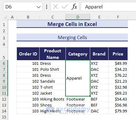
D6:D11 contain the same values:
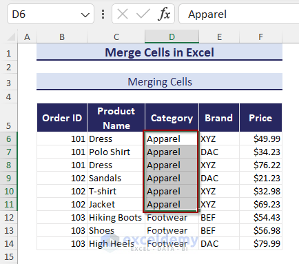
- Merge D6:D11 and it will act like a single cell.
Merge Cells vs Combine Cells
Combining cells means combining the data of multiple cells into one single cell. Merging cells means combining multiple cells into one.
See the difference in the image below:
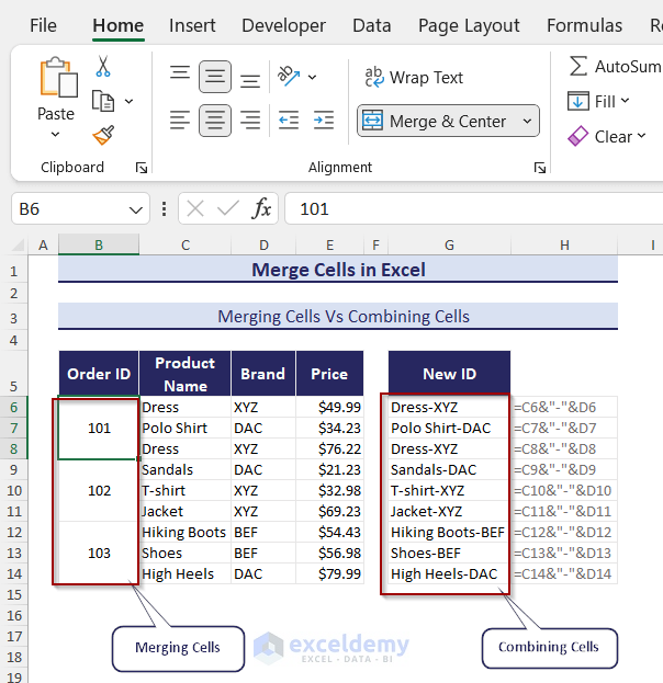
Formulas are used to combine the values of multiple cells.
Cells are merged using the Merge & Center feature, which works for adjacent cells only.
Things You Need to Know Before Merging Cells in Excel
- Merging cells can cause problems when sorting or filtering data.
- If you refer to merged cells in a formula, you may not get the correct output.
- You cannot use the Merge and Center feature directly in an Excel table. You must convert the Table to a range.
- When using Data Validation or Conditional Formatting, avoid merged cells.
How to Merge Cells in Excel – 4 Examples
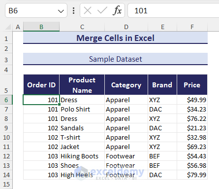
This is the sample dataset.
Example 1 – Merging Cells Using the ‘Merge & Center’ Command
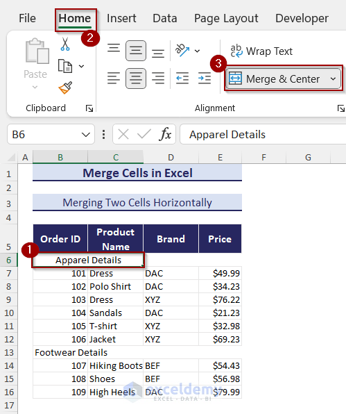
1.1 Merge Two Cells in Excel
To merge B6 and B7:
- Select B6 and B7 cells.
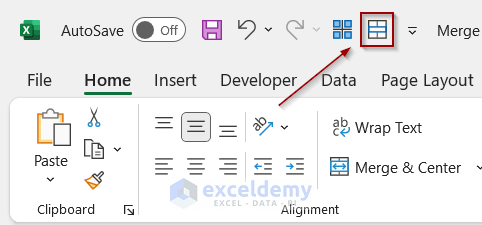
- In the Home tab >> go to Alignment >> click Merge & Center.
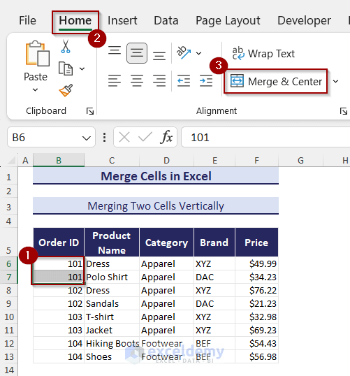
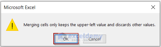
- In the warning message, click OK.
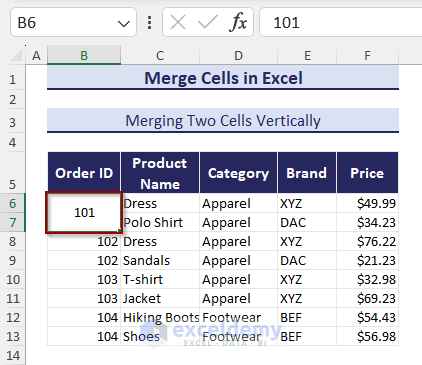
This is the output.
To merge B6 and C6:
- Select B6 and C6.
- In the Home tab >> click Merge & Center.
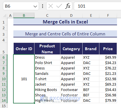
1.2 Merge and Center Cells of an Entire Column in Excel
B6:B14 contains the same value: 101. To merge and center the content of these cells:
- Select B6>> press CTRL + SHIFT + ↓ (Down-Arrow key) to select the column.
- In the Home tab >> Click Merge & Center.
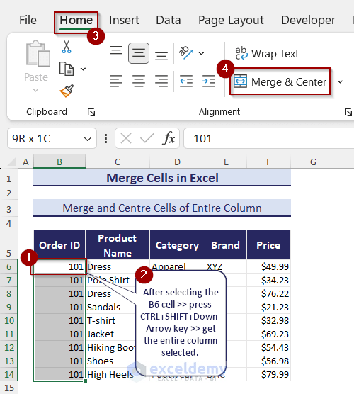
- In the warning message, click OK.
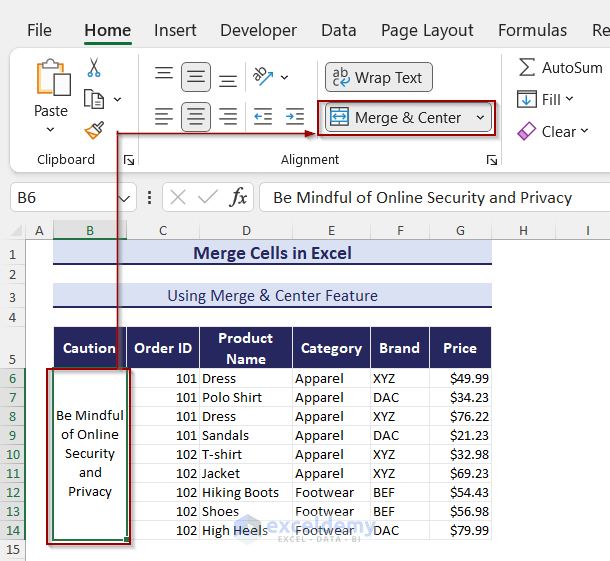
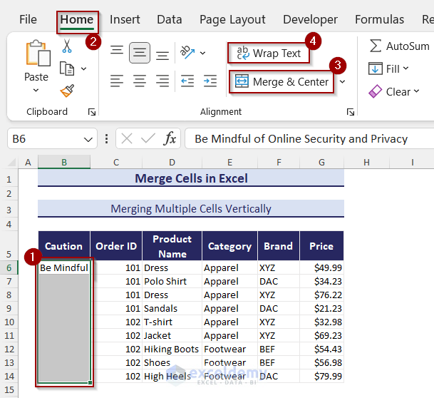
1.3 Merge Multiple Cells Vertically
Cells in column B are empty, except for B6. To merge B6:B14:
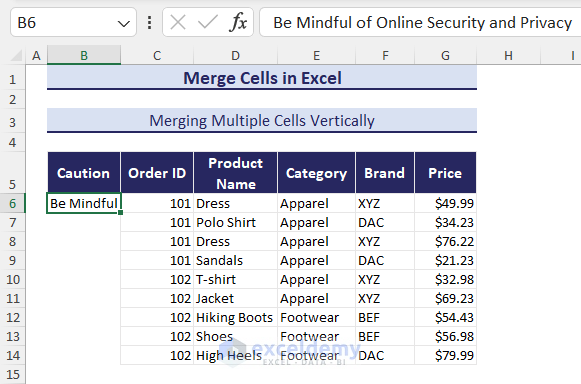
- Select B6:B14 >> in the Home tab >> go to Alignment >> click Merge & Center >> Wrap Text.
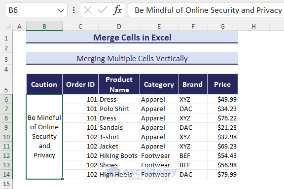
This is the output.
Read More: How to Merge Cells in Excel Without Merging
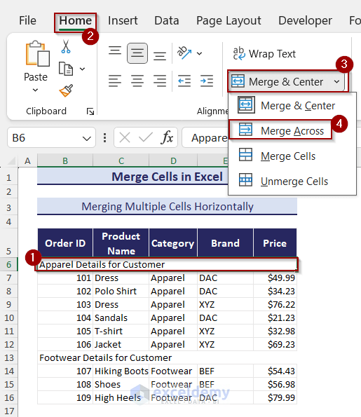
1.4 Merge Multiple Cells in the same Row
- Select B6:F6 >>in the Home tab >> go to Alignment >> Merge & Center >> Merge Across.
- Apply the same procedure to B13:F13.
Adding the Merge & Center Feature to Quick Access Toolbar
- In the Home tab >> go to Merge & Center.
- Right-click an option. Here, Merge Cells.
- Select Add to Quick Access Toolbar.
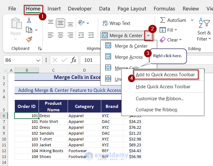
You will see the Merge Cells option in the Quick Access Toolbar.
Read More: How to Move Merged Cells in Excel
Example 2 – Merge Cells Using Keyboard Shortcuts
- To merge cells vertically, select the cells and press ALT+H+M+M.
- To merge cells inthe same row, press ALT+H+M+A.
- To center align, press ALT+H+M+C.
- To unmerge cells, press ALT+H+M+U.
- For Mac, press Control+Option+M to merge cells.
Example 3 – Merging Cells with a VBA Code
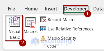
- Go to the Developer tab >> select Visual Basic.
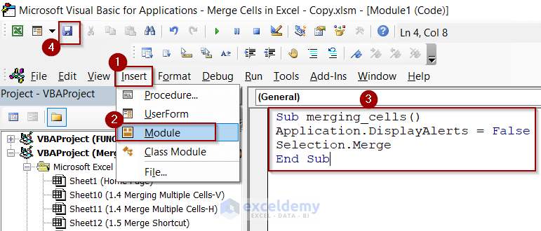
- Select Insert >> Module >> enter the following code in Module 1.
Sub merging_cells()
Application.DisplayAlerts = False
Selection.Merge
End Sub- Save the code.
Use a button to run the code:
- Go back to the worksheet >> Developer tab >> Insert.
- In Form Controls >> Click Button (Form Control).
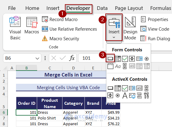
- Drag the Button to the worksheet.
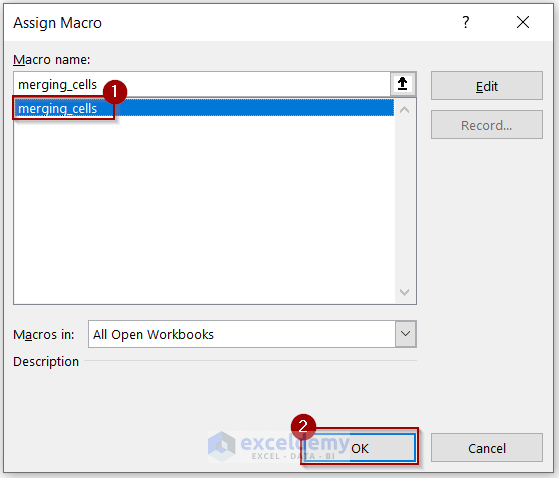
- In Assign Macro, select the sub-procedure merging_cells
- Click OK.
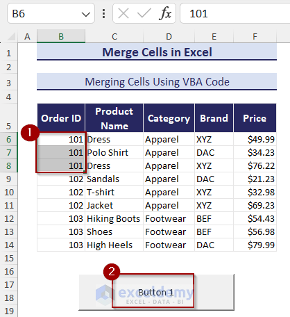
- Select B6:B8 and click Button 1.
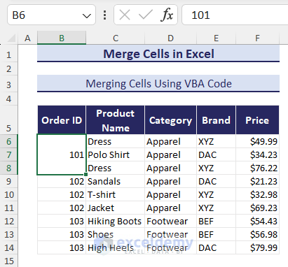
This is the output.
Read More: How to Merge Cells in Excel with Data
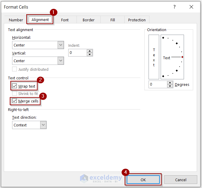
Example 4 – Use the Alignment Feature for Merging Cells
- Select the cells >> press CTRL+1 to open Format Cells.
- Go to Alignment>> Text control >> check Wrap text and Merge cells.
- Click OK.
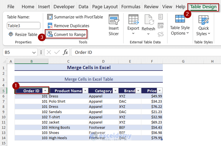
How to Merge Cells in an Excel Table
You can’t merge cells in an Excel table:
Convert the table into a range.

- Select a cell in the table>> go to Table Design >> Tools.
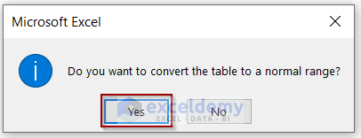
- Click Convert to Range.
- In the message box, click Yes.
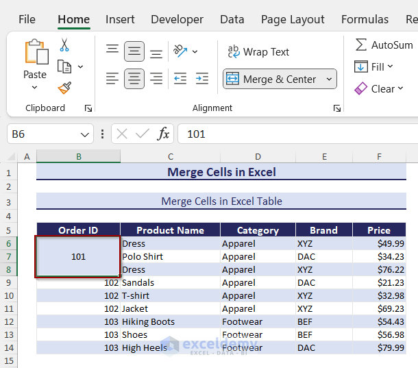
- Use the Merge & Center feature to merge cells.
You can convert this range back into a table by pressing CTRL+T, but the merged cells will automatically be unmerged.
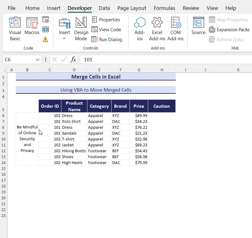
How to Move Merged Cells in Excel
- Go to Developer >>Visual Basic >> Microsoft Visual Basic window.
- Select Insert >> Module >> enter the code in Module 2.
Sub move_merged_cells()
Selection.Cut Range("H6")
End Sub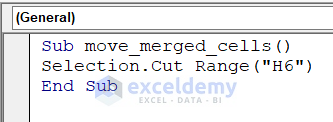
The code will paste your selection in H6.
- Select a merged cell>> Developer >> Macros.
- Select move_merged_cells >> click Run.
The merged cells will move to H6.
Click on the GIF to view it in full-size
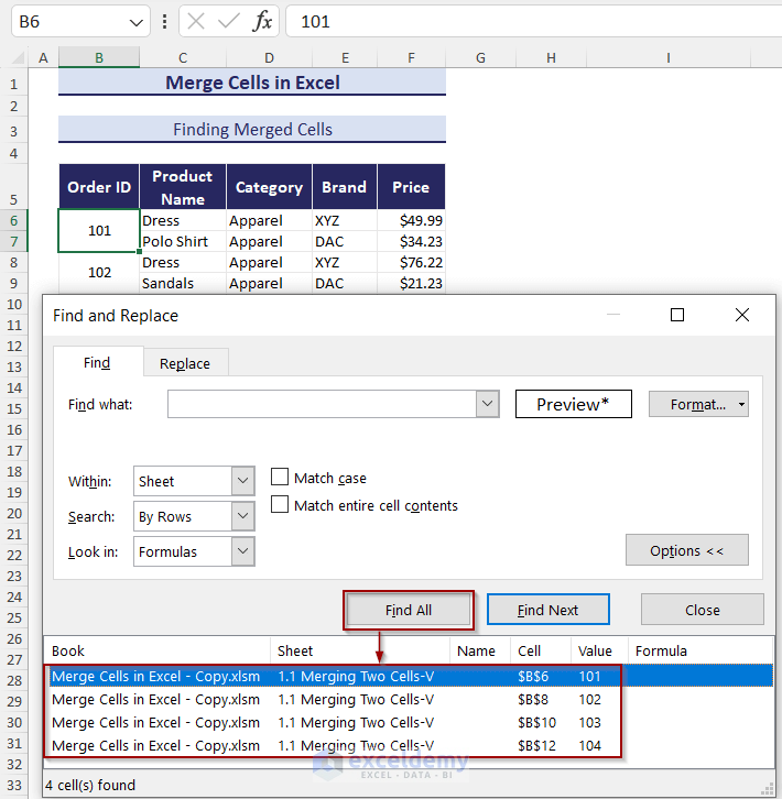
How to Find Merged Cells in Excel
- Press CTRL+F to open the Find and Replace dialog box.
- Click Format.
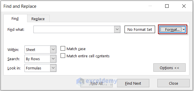
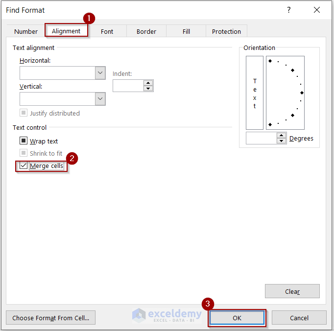
- In Find Format >> go to Alignment.
- In Text control >> check Merge Cells >> Click OK.
- Click Find All.
Merged cells are displayed.
Why Can’t I Merge Cells in Excel?
Possible reasons:
- Cells are part of a table.
- The worksheet is protected: Go to Review >> Protect >> Unprotect Sheet.
- The worksheet is shared: Go to Review >> Protect >> Unshare Workbook.
- The cell is in edit mode: Press ENTER to close the editing mode.
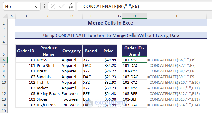
How to Merge Cells Without Losing Data
1. Using Excel Formulas to Merge Two Cells
To merge two non-adjacent cells: B6 and E6 keeping the cell values:
- Go to a blank cell (H6) >> enter the following formula.
=CONCATENATE(B6,"-",E6)- Press ENTER to see the result.
- Drag down the Fill Handle.
You can also use the CONCAT function:
=CONCAT(B6,"-",E6)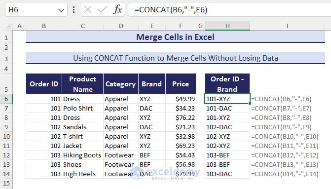
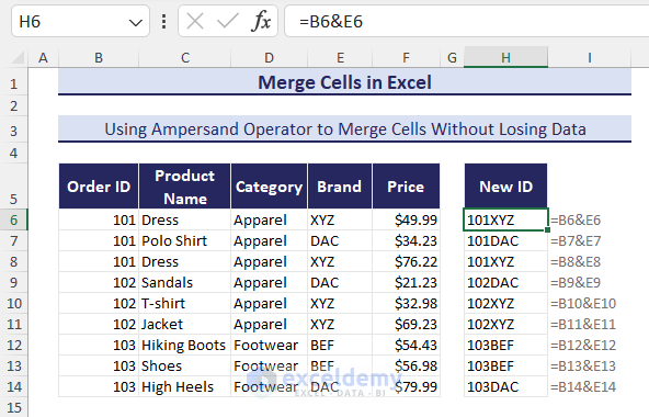
Alternatively, use the ampersand operator to connect two cells keeping the values.
- Go to H6 >> enter the formula below >> press ENTER.
=B6&E6- Drag down the Fill Handle.
2. Applying the TEXTJOIN Function to Combine Multiple Cells
To combine B6:E6:
- Use the formula:
=TEXTJOIN(",",TRUE,B6:E6)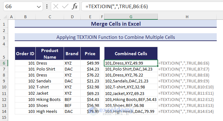
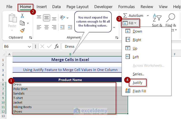
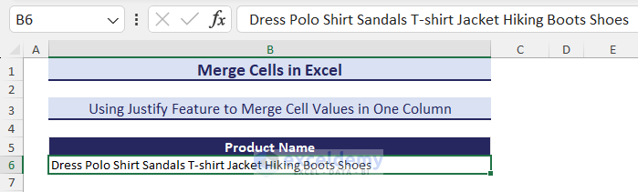
3. Merge Cells in One Column Using the Justify Feature
- Expand column B so that all values (B6:B12) are displayed.
- Select B6:B12>> Go to the Home tab >> Editing >> Fill >> Justify.
Click on the image to have a detailed view
This is the output.
Read More: How to Merge Data from Multiple Workbooks in Excel
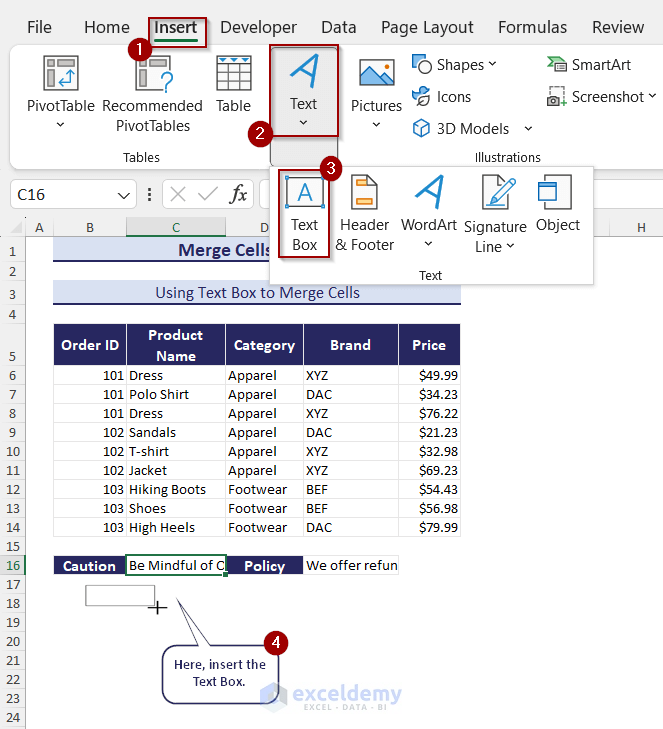
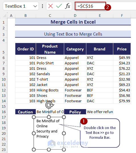
An Alternative to Merging Cells in Excel: Inserting a Text Box
- Go to the Insert tab >> Text >> select Text Box.
- Drag the Text Box to the sheet.
- Double-click the Text Box >> go to the Formula Bar.
- Enter =$C$16 >> press ENTER.
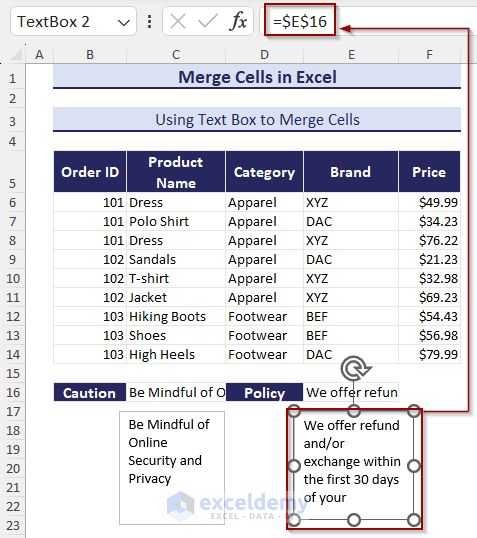
- Insert another Text Box >> go to the Formula Bar >> enter =$E$16 >> press ENTER.
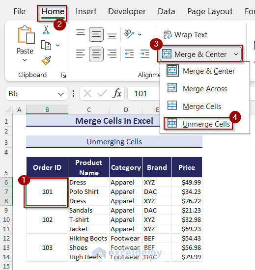
How to Unmerge Cells in Excel
- Select the merged cells (B6:B8) >> Home >>Merge & Center >> Unmerge Cells.
This is the output.
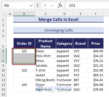
If you unmerge cells, the value takes the place of the uppermost left cell. The other cells remain empty.
Excel Merge Cells: Knowledge Hub
<< Go Back to Merge in Excel | Learn Excel
Get FREE Advanced Excel Exercises with Solutions!
