How to Merge Datasets in Excel (5 Easy Methods)

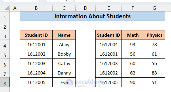
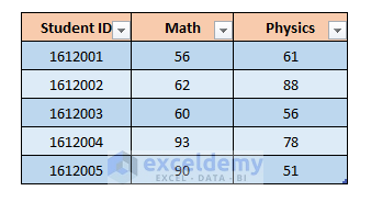
The below dataset contains a table displaying, Student IDs and Names and another table containing Student IDs, Math, and Physics Scores. We will merge the lists and show them in a new single list.

Method 1 – Using VLOOKUP

Steps:

• To make a new list:
  • Copy the left table and the heading of the Math and Physics Column of the right table.
  • Paste it into a convenient place. We have placed it just below the old tables.

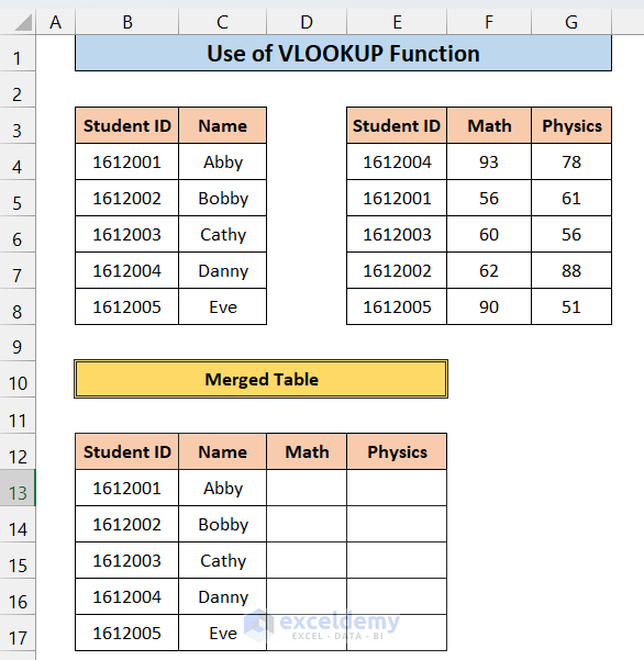
In cell D13, we will search for the Math scores of Abby.

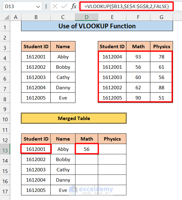
• Enter the following formula:

Here,

• $B13 is the value to be searched.
• $E$4:$G$8 is the range where the value will be searched in the first column.
• 2 is the column number from where data will be extracted (Math has column number 2).
• FALSE is for exact matching.

• Lock the reference cells, as it is very important to copy the cell formula.
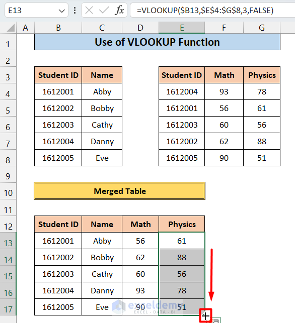
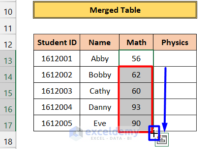
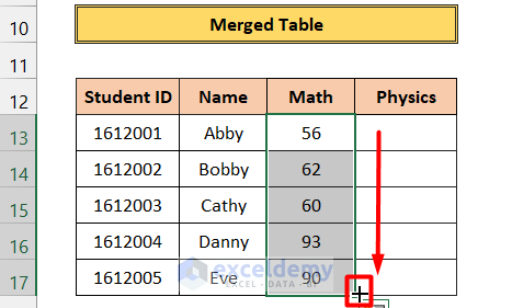
• Use the Fill Handle to AutoFill up to D17.

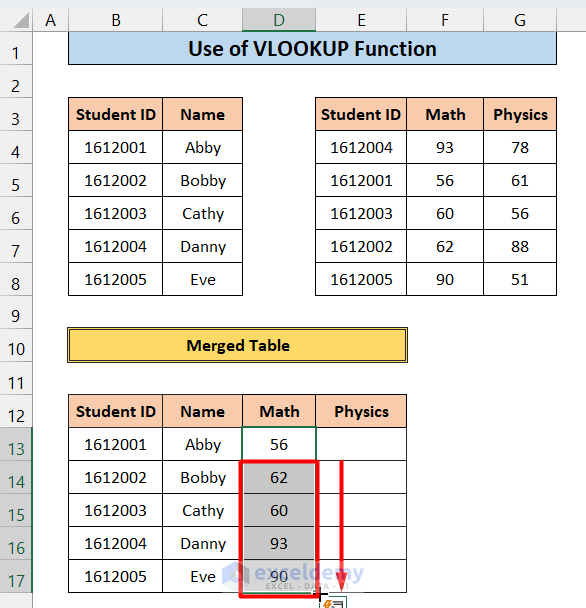
You can see that we have the Math scores of other corresponding students as well.

• To find the Physics score, go to cell E13 and enter the same formula:

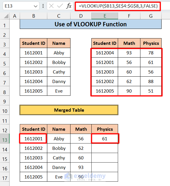
• Use the Fill Handle to AutoFill up to E17

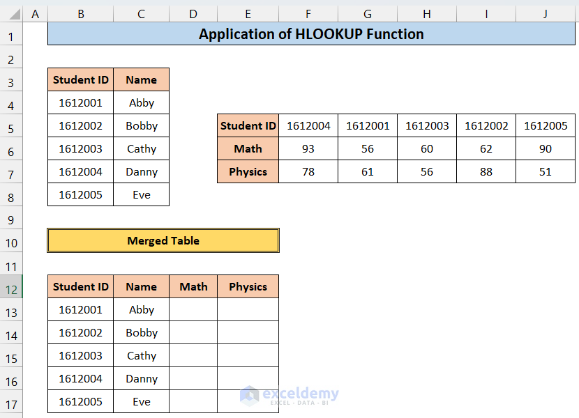
Method 2 – Applying Excel HLOOKUP 

Steps:

• Copy the first list and the header column in the second list and paste them below, like this.

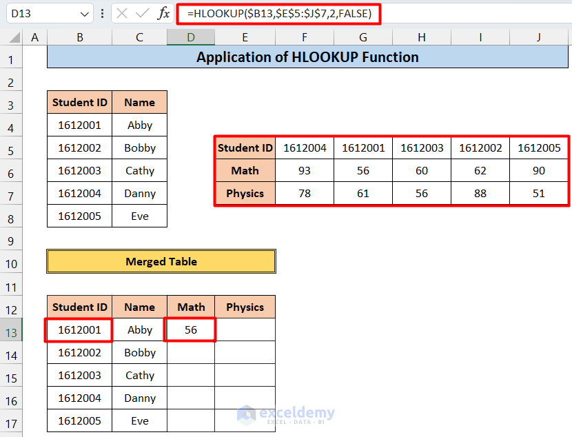
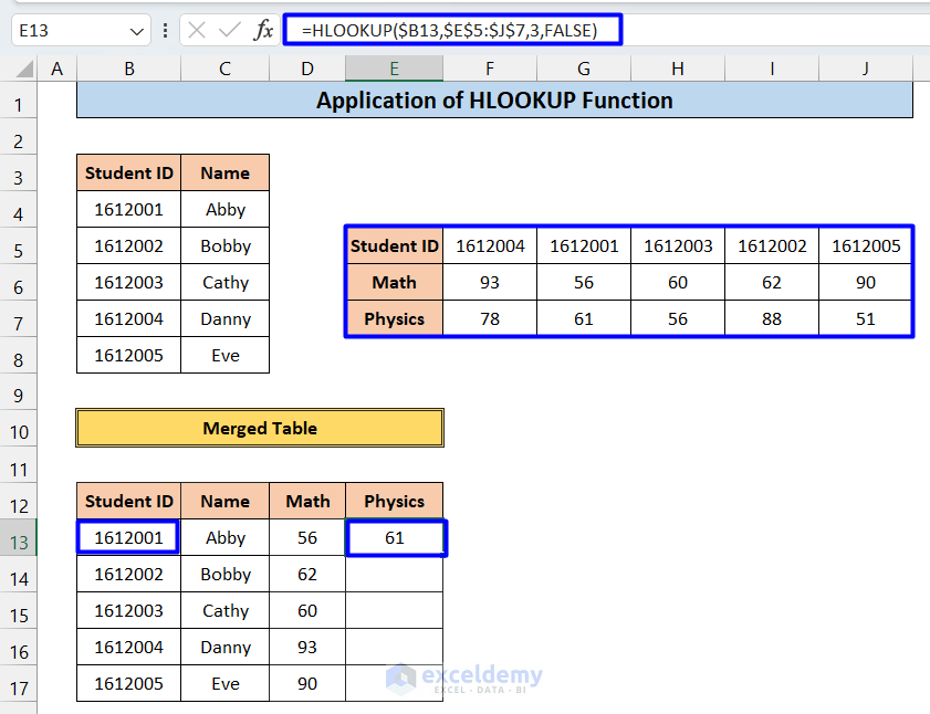
• Enter the following formula in cell D12:

Here,

• • $B13 is the value to be searched
  • $E$5:$J$7 is the range where the value will be searched in the first column
  • 2 is the row number from where data will be extracted (Math has the column number 2)
  • FALSE is for exact matching.
• Click Enter, and you will get the following result.

• Use the Fill Handle to AutoFill up to D17.

• Enter the following formula in cell E13:

• Click Enter, and the result will look like this.

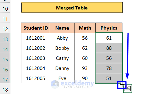
• Use the Fill Handle to AutoFill up to cell E17. You will get our desired final result.

Method 3 – Combining INDEX & MATCH Functions

3.1 Single Column

Steps:

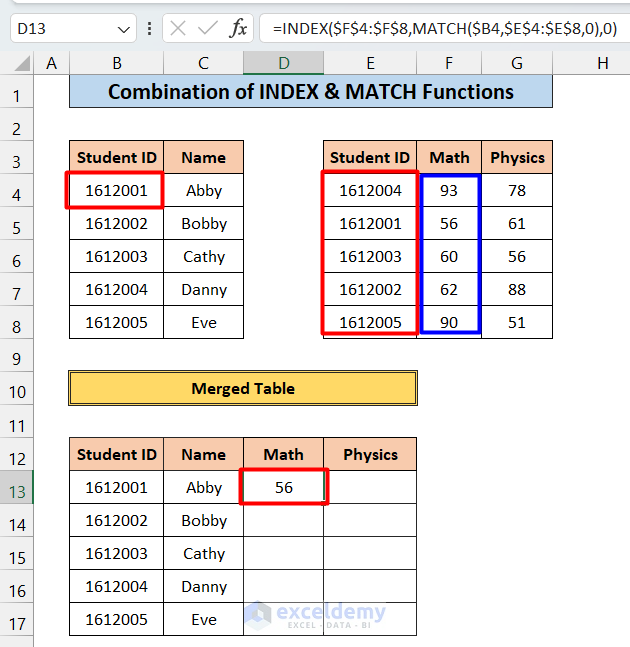
• Enter the following formula in cell D13:

Here,

• • $F$4:$F$8 is the return range(Math column in List 2)
  • $B4 is the lookup value(1612001)
  • $E$4:$E$8 is the look-up range(Student Id Column in List 2)
  • 0 is for the exact match
• Press Enter, and you should get the following result

• Drag down the Fill Handle on cell D13 to D17 to get the remaining corresponding cell values.

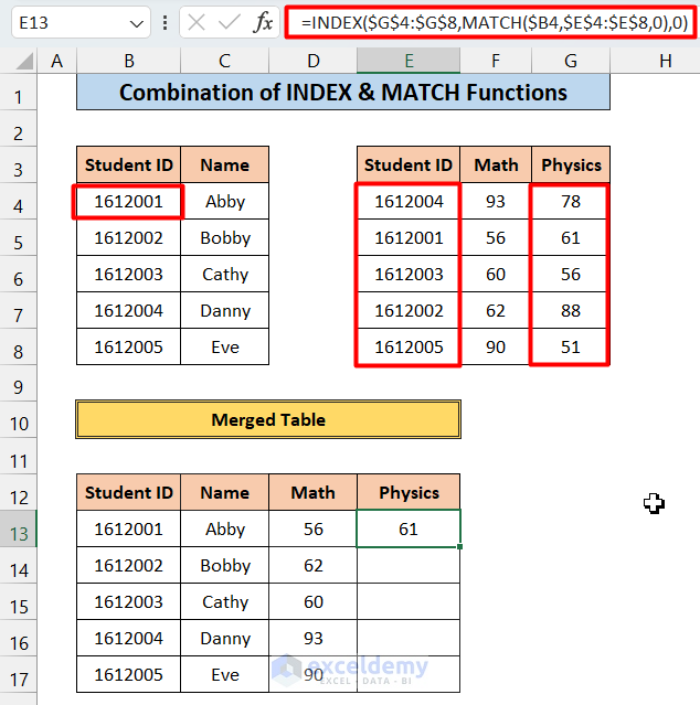
• To get the cell values in the Physics column, enter the following formula in E13:

Here,

• $G$4:$G$8 is the return range(Physics column in List 2)
• $B4 is the lookup value(1612001)
• $E$4:$E$8 is the look-up range(Student Id Column in List 2)
• 0 is for the exact match

You should get the following result:

• Drag down the Fill Handle on the cell E13 to E17 to get the remaining corresponding cell values.

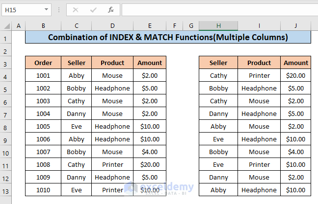
3.2 Multiple Columns

Steps:

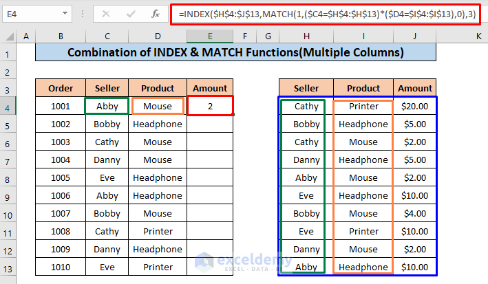
• Enter the following formula in cell E4:

Here,

• $H$4:$J$13 is the lookup table (2nd data table)
• $C4=$H$4:$H$13 is equating to the value of cell C4 ( “Abby”) in the H4:H13 column( Seller column in the 2nd list).
• $D4=$I$4:$I$13 is equating the value of cell D4 ( “Mouse”) in the I4:I13 column( Product column in the 2nd list)
• 0 is for exact matching
• 3 is for returning the value from the 3rd column of the 2nd list.

Lock the cell reference mentioned above accordingly otherwise, we will not be able to copy the formula.

• Drag down the Fill Handle on cell E4 to E13 to get the remaining corresponding cell values.

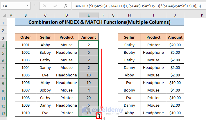
• After formatting the cells we will get our desired final result.

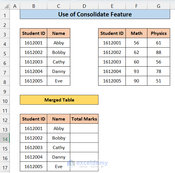
Method 4 – Using the Consolidate Feature 

Steps:

• Copy the Student ID and Name columns. Create a new column named Total Marks.

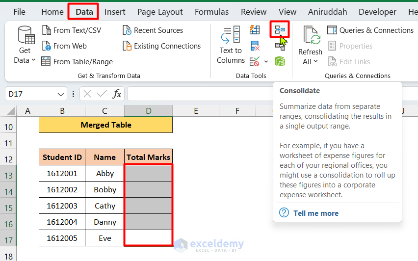
• Select cell range D13:D17.
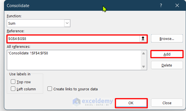
• Go to the Data. Select the Consolidate feature. (See image below)

• In the dialogue box, choose the function Sum.
• Select the reference for the marks of Math.
• Click Add.

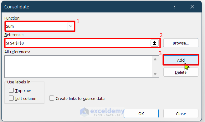
• Add the marks for Physics.
• Click OK

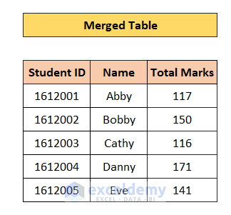
You will have the following result.

Method 5 – Using the Excel Power Query 

Steps:

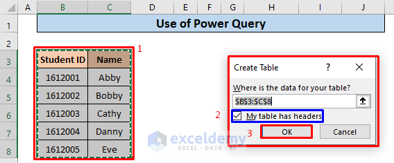
• Select cell range B3:C8.
• Press CTRL+T.
• Create Table box will appear. Check the My table has headers.
• Click OK.

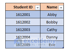
• Here, Excel will generate a table for you like below.

• Create a table for G3:I8 like the one below.

• Give the tables a name. We named the first one St_Name and the 2nd one Numbers.

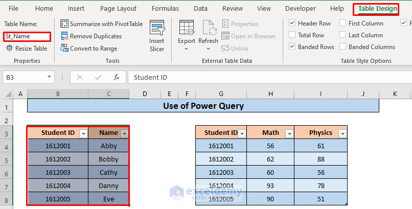
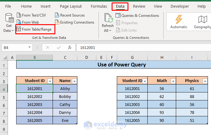
• Select any cell in Table St_Name and go to the Data tab. Choose From Table/Range in the Get & Transform Data group.

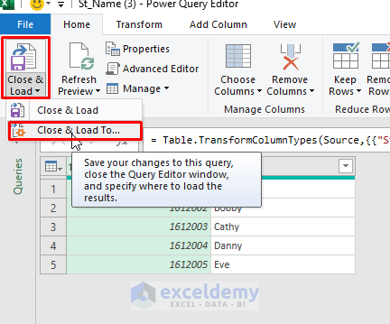
• A Power Query editor will open. Click on the Close & Load dropdown arrow, and select the Close & Load To option like in the figure below.

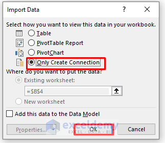
• A new dialogue box named Import Data will open.  Select Only Create Connection, and click OK

• Do the same for Table Numbers. You will see a query tab on the right side of the screen. Here, you will see 2 queries. (See the figure)

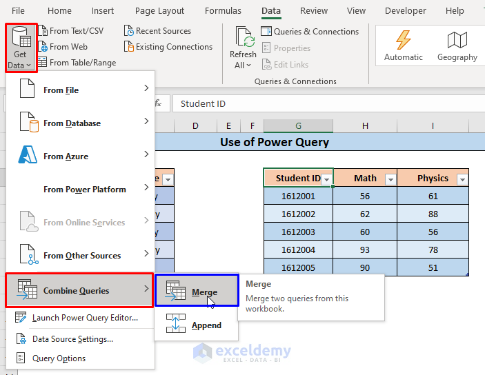
• Go to the Data tab and from the Get Data drop-down list, select Combine Queries > Merge like the figure below.

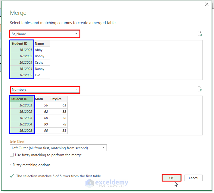
• A new window named Merge will open. From the dropdown lists, choose the following, as shown in the figure. Now, you have to select the common column. So select Student ID in both tables, and they will be highlighted in green. Now click.

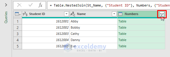
• A new window named Queries will open. In the Numbers column, click on the icon(Expand radio button), as shown in the figure.

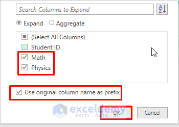
• Another window will open. Uncheck Student ID and check to use the original column name as a prefix, and click OK.

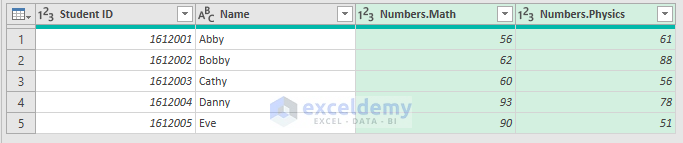
• You will see a Math and Physics column showing in the Queries Window.

• To import this table, click on the Close & Load drop-down arrow and choose Close and Load To…
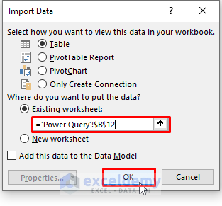
• In the Import Data window, select Table and Existing worksheet.
• Choose a suitable position for your merged table. We have selected B12.
• Click OK.

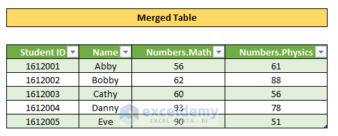
• You will have your desired merged data in an Excel table.

Things to Remember

• Use the first two methods for a quick merging of data sets.
• Use the Power Query method if you have a large data set in a table format.
• Use the Consolidate method to get the sum or average of the data sets.

Download the Practice Workbook

Download this workbook to practice.

<< Go Back to Cells | Merge | Learn Excel