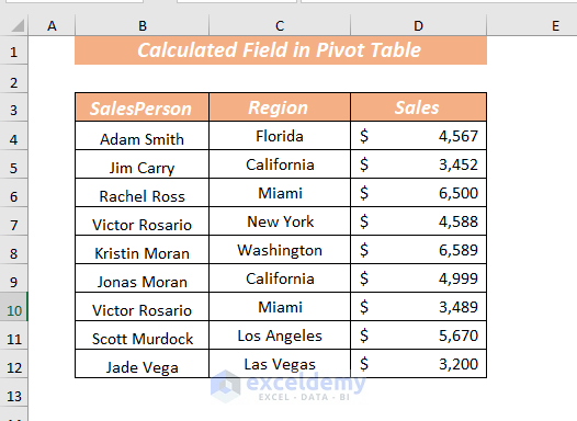
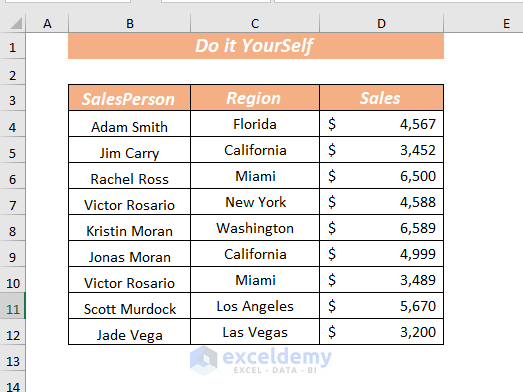
We’ll use a sample dataset that represents the sales information of a particular salesperson. The dataset has 3 columns: SalesPerson, Region, and Sales.
How to Use a Calculated Field in a Pivot Table
Part 1 – Create a Pivot Table
We’re going to use the dataset given below.
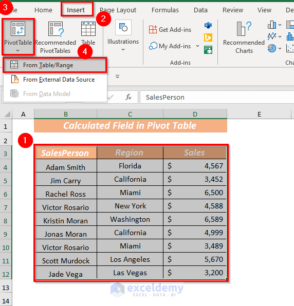
- Select the cell range from where you want to create a Pivot Table. We selected the cell range B3:D12.
- Open the Insert tab and under PivotTable select From Table/Range
- A dialog box will pop up. Choose the location or cell to place your PivotTable. We selected New Worksheet.
- Click OK.

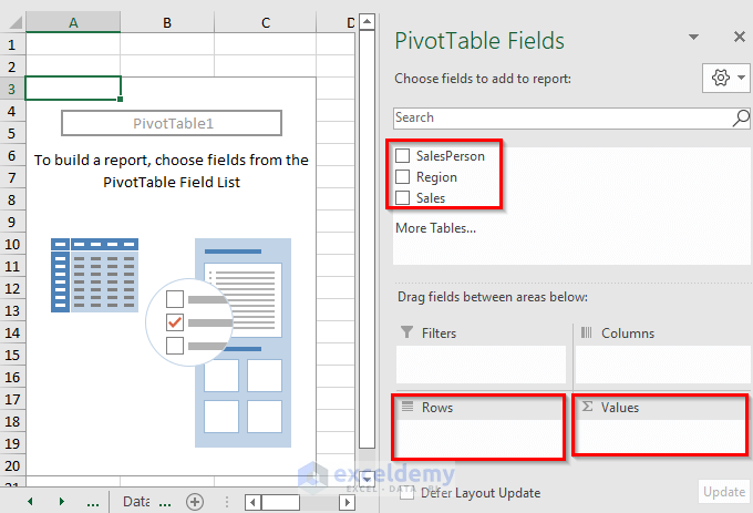
- A new sheet with the PivotTable will open.
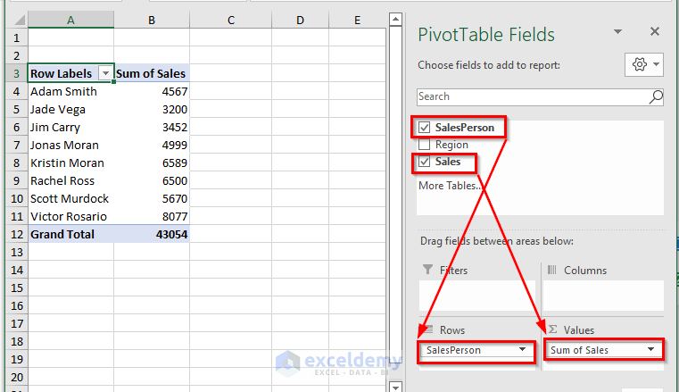
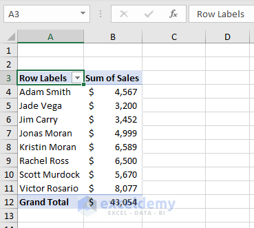
- Choose the fields from PivotTable Fields that you want to display in the PivotTable layout. We selected the SalesPerson in Rows and Sales in Values.
- You will get the selected fields in the PivotTable layout.
Part 2 – Inserting a Simple Calculated Field in a Pivot Table
We want to add a field named Bonus depending on the Sales information. The bonus amount will be 5% of the sales.
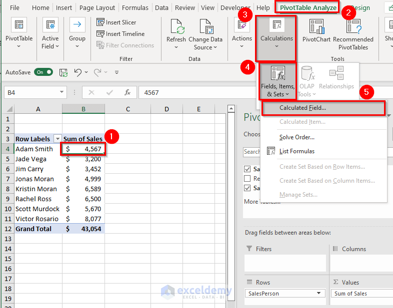
- Select B4 from the Pivot Table.
- Open the PivotTable Analyze tab and go to Calculations.
- From Fields, Items, & Sets, select Calculated Field
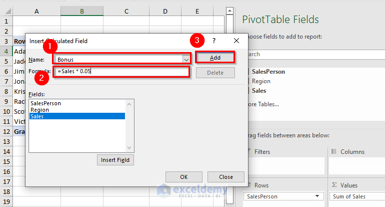
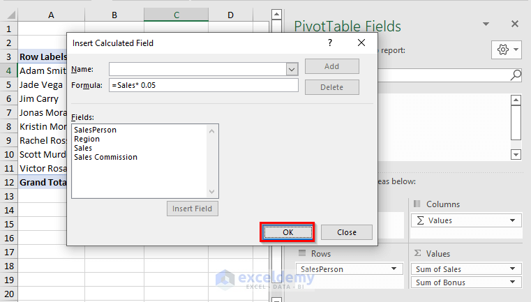
- A dialog box will pop up. Insert a Name and a Formula. We used Bonus in Name.
- Insert the following formula in Formula.
=Sales*0.05- Click Add.
- Click OK.
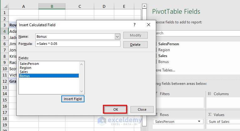
- You will get the Calculated Field named Bonus in the PivotTable.
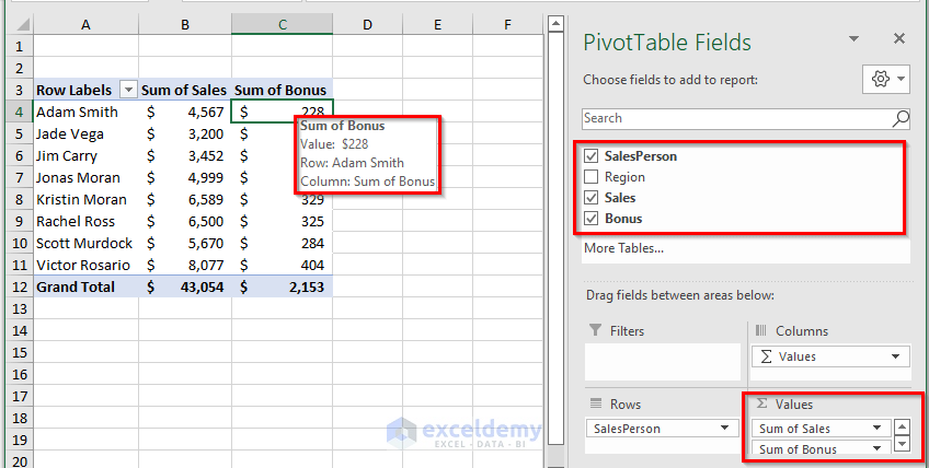
- All Bonuses are calculated automatically.
Part 3 – Adding Complex Calculated Fields in Pivot Table
We’ll calculate the Commission based on Sales. If a sales amount is greater than (>) $5,000 the salesperson will get 8% of the commission.
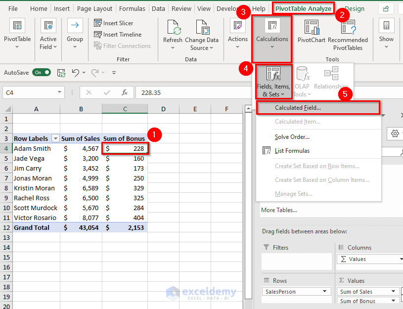
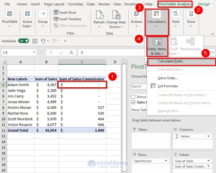
- Select any cell from the Pivot Table. We chose C4.
- Open the PivotTable Analyze tab, go to Calculations, and from Fields, Items, & Sets, select Calculated Field
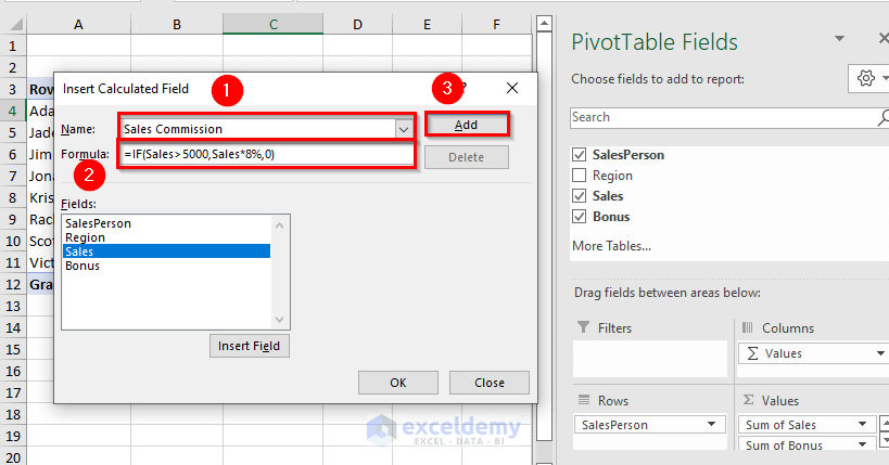
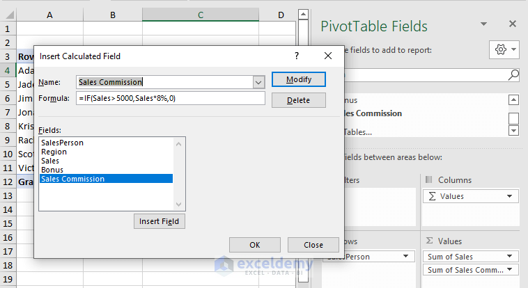
- A dialog box will pop up. From there insert Name and Formula. We put Sales Commission in Name.
- Use the following formula in Formula.
=IF(Sales>5000,Sales*8%, 0)- Click Add.
- Click OK.
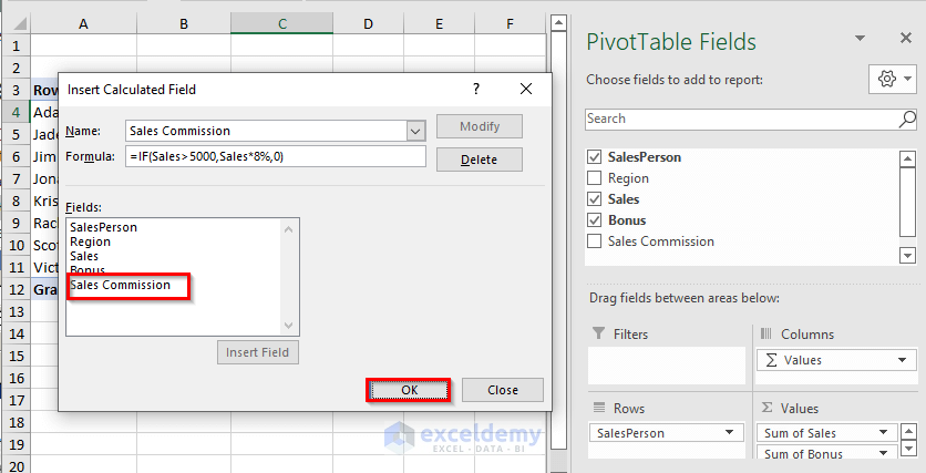
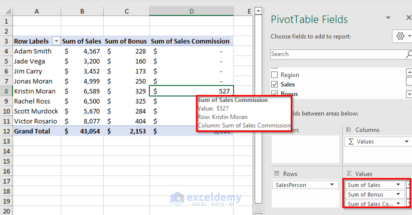
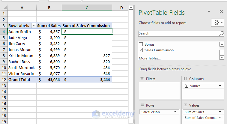
- You will get the Calculated Field named Sales Commission in the PivotTable.
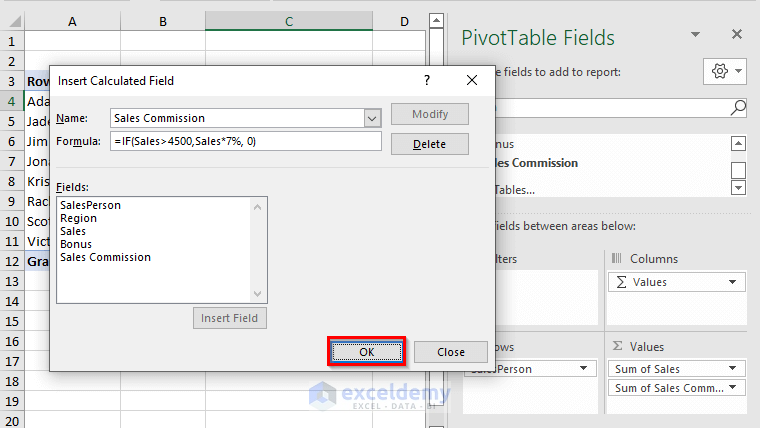
Part 4 – Modify an Existing Calculated Field
We want to modify the field Sales Commission. We want to provide a 7% commission where the sales value is greater than $4,500.
- Select any cell from the Pivot Table.
- Open the PivotTable Analyze tab, go to Calculations, choose Fields, Items, & Sets, and select Calculated Field.
- A dialog box will pop up. Select Sales Commission from Name to see the existing Formula.
- Replace the formula with:
=IF(Sales>4500,Sales*7%, 0)- Click Add.
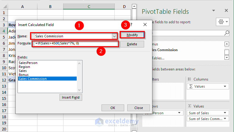
- Click OK.
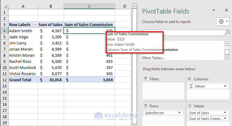
- You will get the modified values in the Calculated Field named Sales Commission in the PivotTable.
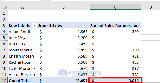
Part 5 – Drawback of Calculated Fields in Pivot Table
Look at the Sum of Sales Commission which shows $3,014. Let’s calculate the SUM manually using the SUM function.
- Select cell C13.
- Insert the following formula.
=SUM(C4:C11)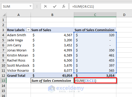
- Press the Enter key to get the SUM.
- You will get the SUM of the Sales Commission.
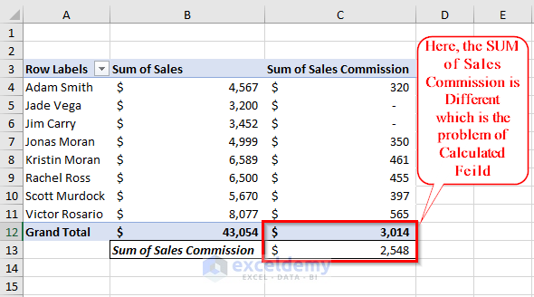
The Grand Total from the Calculated Field is 3,014 and the Grand Total we got from the SUM function is 2,548.
This means the Grand Total of the Calculated Field is incorrect for the Sales Commission field. The Grand Total is not the SUM but the 7% of the Grand Total of Sales, because the Calculated Field uses the same calculation in the SubTotal and Grand Total rows.
Part 5.1 – Ways to Avoid Calculation Problem of Calculated Field
You can use the Filter option to avoid the calculation problem.
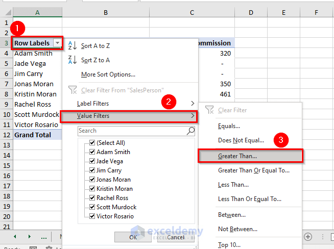
- Select the Row Labels and expand the Filter options.
- From Value Filters, select Greater Than.
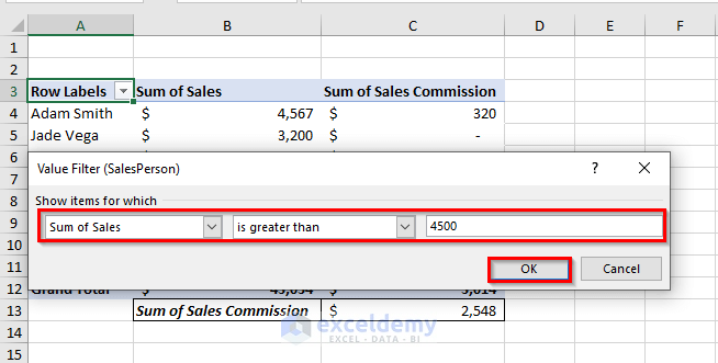
- In Show items for which, provide the conditions you already used in your Calculated Field. We selected “Sum of Sales,” “is greater than,” and “4500”.
- Click OK.
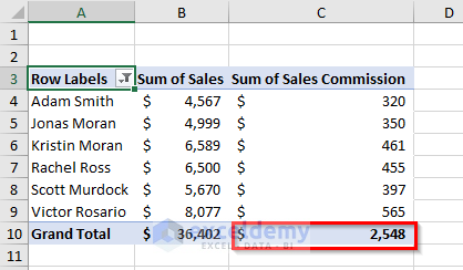
- You will get the Grand Total of the values which met the condition applied on the Calculated Field.
- The Grand Total of Sales Commission is 2,548.
- In cell C13, use the following formula.
=SUM(C4:C9)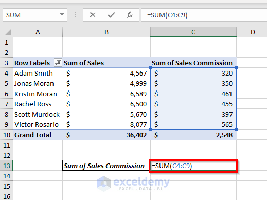
- The SUM function will add all the available values of the selected range C4:C9.
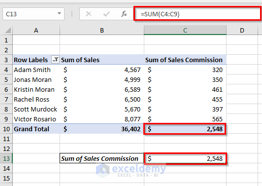
- Both Grand Total and SUM are equal.
You can also remove the Grand Total from the sheet.
- Right-click on Grand Total.
- Select Remove Grand Total.
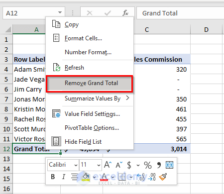
- The Grand Total is removed from the sheet.
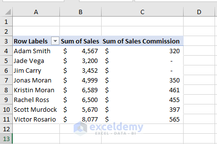
You can calculate the Grand Total outside the PivotTable just as we did to get the SUM of the Sales Commission.
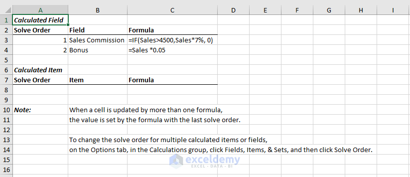
Part 6 – Get a List of All the Calculated Field Formulas
- Open the PivotTable Analyze tab, go to Calculations, go to Fields, Items, & Sets, and select List Formulas.
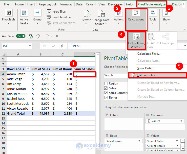
- All the used formulas will appear in a new sheet.
Part 7 – Temporarily Remove a Calculated Field
We want to remove the Sum of Bonus Calculated Field temporarily.
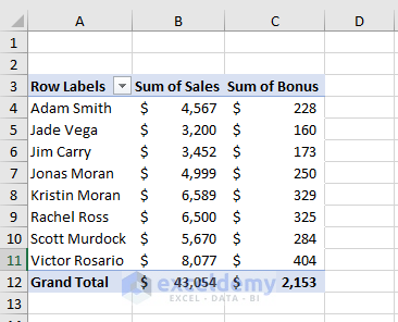
- Select any cell from the Calculated Field that you want to remove. We selected cell C3.
- Right-click and select Remove “Sum of Bonus”.
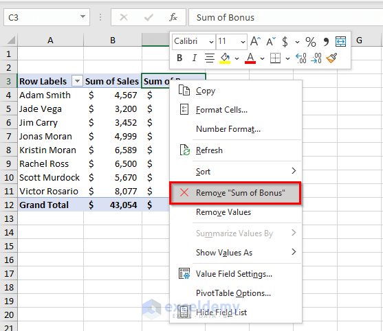
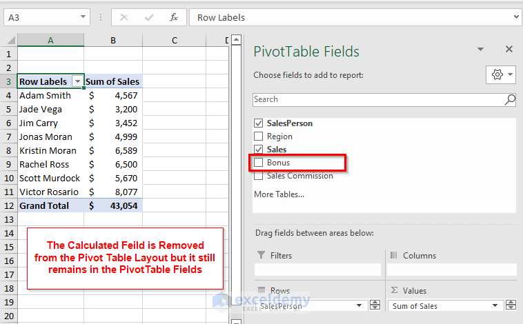
- The Calculated Field Sum of Bonus is removed.
- Though the Sum of Bonus field is removed from the PivotTable layout, it is still available in PivotTable Fields. You can use it again if you want.
You also can uncheck the Calculated Field from the PivotTable Fields to remove the Calculated Field temporarily.
Part 8 – Permanently Remove a Calculated Field from a Pivot Table
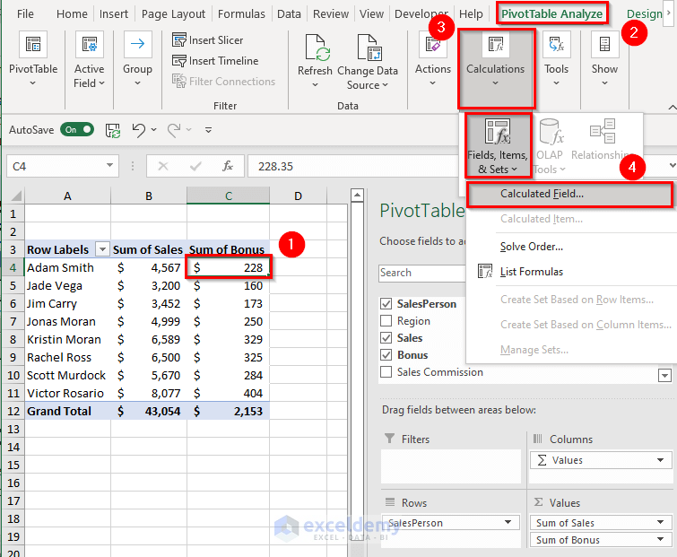
- Select any cell from the Calculated Field that you want to remove permanently.
- Open the PivotTable Analyze tab, go to Calculations, then, from Fields, Items, & Sets, select Calculated Field.
- A dialog box will pop up. Select Bonus in Name to see the existing Formula.
- Click on Delete.
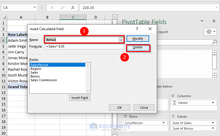
- Click OK.
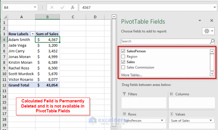
- The Sum of Bonus field is removed permanently from the PivotTable layout as well as from the PivotTable Fields.
Practice Section
We’ve provided a practice sheet in the workbook to practice these explained examples.

Download the Practice Workbook
How to Use Calculated Field in Excel Pivot Table: Knowledge Hub
<< Go Back to Pivot Table Calculations | Pivot Table in Excel | Learn Excel
Get FREE Advanced Excel Exercises with Solutions!

Very Good Condition & Application of Excel Pivote
Hello Fazlay Rabby
Thanks for your compliment! You are very welcome. We are glad that you found the article helpful.
Regards
Lutfor Rahman Shimanto
ExcelDemy
Good morning, quick question, is there a way to create a calculated field in a pivot table where the source data is as below:
Columns (A/B/C)
Column A: contains the metric called “Value” which shows the total sales value
Column B: contains the metric called “Volume” which shows the total sales Volume
Column C: contains sales person name
I need to know for which sales person the average Sales value.
Example:
Value – 100 – John
Volume – 10 – John
Value – 500 – Andrew
Volume – 100 – Andrew
I need a pivot table which shows the average of 10 for John and the average of 5 for Andrew.
Thank you,
Andrei
Hello Andrei,
Good morning! Yes, you can achieve this by creating a calculated field in the Pivot Table. Here’s how you can set it up:
Set Up Your Pivot Table:
1. Select your source data and create a Pivot Table.
2. Place Sales Person (Column C) in the Rows section.
Create the Calculated Field:
1. Click anywhere inside the Pivot Table.
2. Go to the PivotTable Analyze tab on the ribbon >> from Fields, Items & Sets >> select Calculated Field.
3. In the dialog box, give your calculated field a name, like “Average Sales Value.”
4. Enter the formula: = Value / Volume.
Adjust the Values Area: Add the calculated field to the Values area. It will automatically calculate the average sales value for each salesperson.
Regards
ExcelDemy
Hi There,
Thanks for all this explanation.
On my excel file/pivot table, the entry “Calculated field” is not accessible. I did not find the reason for that. Any clue?
Thx
Nicolas
Hello Nicolas,
You’re welcome! If the Calculated Field option is grayed out or inaccessible in your Pivot Table, here are a few possible reasons and solutions:
Check the Pivot Table Type: If your Pivot Table is based on an OLAP data source (Power Pivot or external data model), the Calculated Field option will be disabled. Instead, you need to use Measures (DAX formulas) in Power Pivot.
Ensure You’re in the Correct Context: Click inside the Pivot Table before trying to access the Calculated Field option under the PivotTable Analyze → Fields, Items & Sets menu.
Verify Your Data Source: If your Pivot Table is using data from an external source, some features may be restricted.
Try Refreshing the Pivot Table: Sometimes, a simple refresh (Right-click → Refresh) can help unlock options.
If you’re still facing issues, let me know more details about your data source and Excel version, and I’d be happy to help!
Regards
ExcelDemy