How to Get a Count in Excel Pivot Table Calculated Field

The Calculated Field is a powerful feature used to analyze the values of some other fields in an Excel Pivot Table using formulas. By default, the Calculated Field works on the sum value of the other Pivot Table field. But by using a simple trick, we can obtain a count value instead of a sum.

Creating a Pivot Table

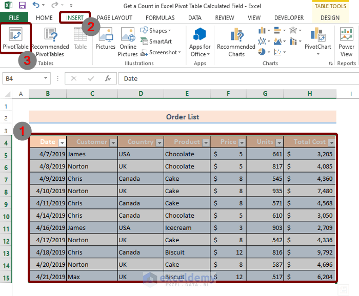
Below, we have a sample order list in Excel Table form. We will turn this table into a Pivot Table to demonstrate how to use Calculated Field to count.

STEPS:

• Select the Excel table.
• Go to the INSERT menu from the main ribbon.
• Click on the PivotTable option.

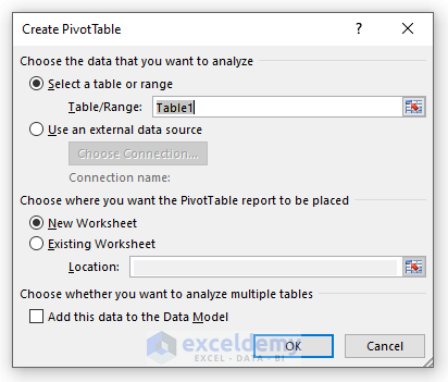
A dialog box named Create Pivot Table will appear.

• Change the Table Name and create a Pivot Table either in a New Worksheet or in an Existing Worksheet, as you please.
• Click OK.

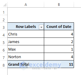
• From the Pivot Table Fields dialog box, select the fields that you want in your Pivot Table. For example, drag the Customer field to the ROWS column and the Date field to the VALUES column.

The Pivot Table is generated.

An Issue with the Pivot Table Calculated Field

The main issue with using the Calculated Field is that it works with the SUM value of the other fields in the Excel Pivot Table.

For example, say we want to see the number of order dates for each customer name. So we have a column that shows the corresponding order dates for each customer.

The number of order dates is a count value. But the serial number of an individual date is a much bigger numerical value than the count value.

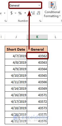
So the Calculated Field considers the serial numbers of the individual dates rather than the count value of the order dates.

Illustrating the Problem

Let’s create a new Calculated Field to illustrate the problem.

STEPS:

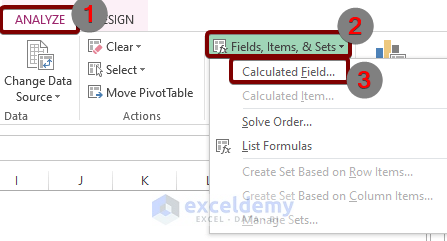
• Click on a cell of your Pivot Table.
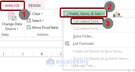
• Go to the Analyze menu.
• From the Calculations group, select Fields, Items, & Sets.
• Click on Calculated Field from the drop-down list.

A new dialog box, Insert Calculated Field, will appear.

• In the Name box, insert >3 (to see all the dates with a count greater than 3).
• In the Formula box, type equal (=), then double click on Date from the Fields list, then type >3.
• Click OK.

So the whole formula is:

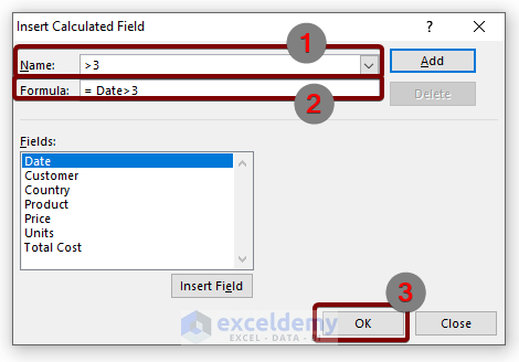
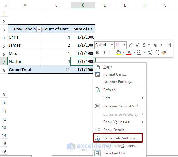
The new field shows the date instead of count values. To change it:

• Right-click on a cell and select Value Field Settings from the context menu.

The Value Field Settings window will open.

• Click the Number Format button at the bottom.

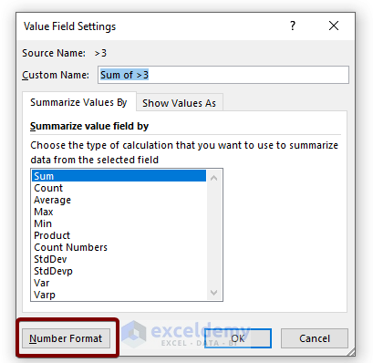
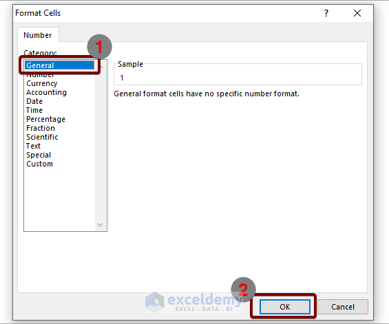
The Format Cells dialog box will appear.

• Select General and click the OK button.

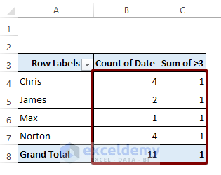
A new field is added to the Pivot Table named Sum of >3.

The values in the column are all 1. But this is incorrect. According to the formula set in the Calculated Field dialog box, the digit 1 should represent date counts greater than 3 and the digit 0 should represent the counts less than 3.

Calculated Field is not considering the count value of the Count of the Date column. Instead, it is using the serial number of the individual dates, which are much larger than 3, hence the cells in the Sum of >3 column are all showing 1.

Read More: Calculated Field Sum Divided by Count in Pivot Table

Get a Count in Excel Pivot Table Calculated Field

A – Add a Helper Column to the Source Data

As the Calculated Field can’t read the count value of the fields generated by the Pivot Table, we will add an extra column to the source data named Helper.

This extra column will copy the values of the count value of another Pivot Table field. Thus, using the value of the Helper column, the Calculated Field will show the count value properly.

STEPS:

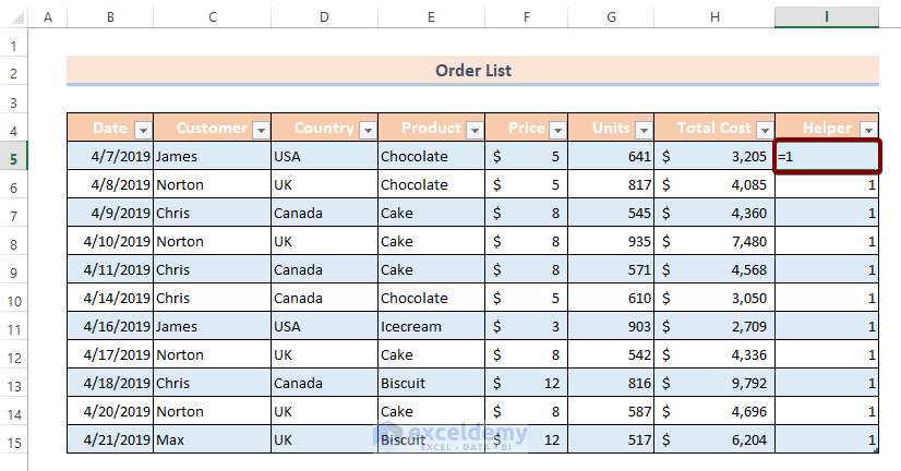
• Add an extra column to the source data called Helper. It will automatically get updated, as the source data table is an Excel Table.
• In cell I5, enter the following formula and press ENTER:

The rest of the cells of the Helper column will automatically copy the formula.

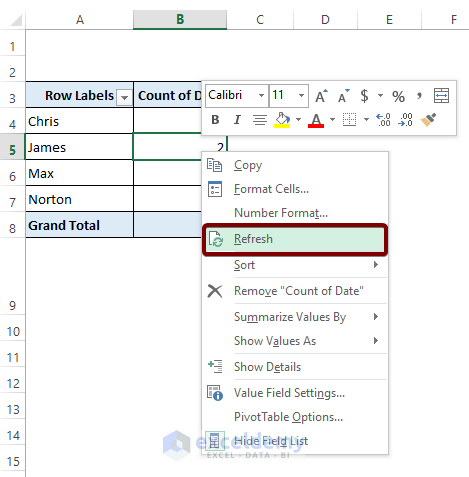
This newly added column hasn’t been updated to the PivotTable Fields list.

• To update, right-click on a cell of the Pivot Table and click on Refresh.

The Helper field appears in the PivotTable Fields list.

• Mark the Helper field and drag it to the VALUES column.

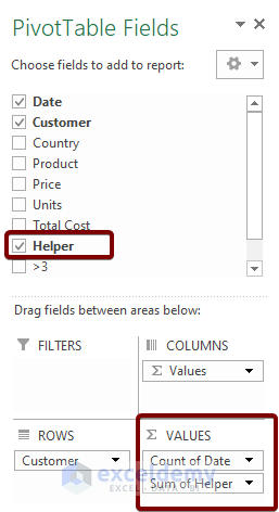
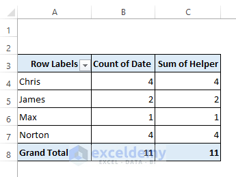
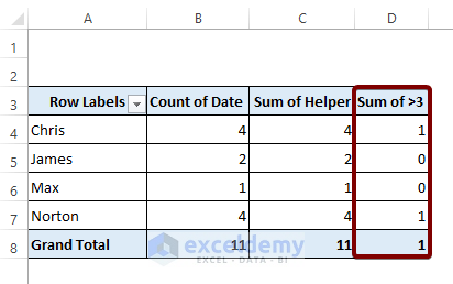
The Helper field is updated with the name Sum of Helper. This field has copied all the data from the Count of Date column.

B – Create a Calculated Field to Get the Count

Now let’s create another Calculated Field that will show the date counts actually greater than 3.

STEPS:

• Click on a cell of the Pivot Table.
• Go to the Analyze tab.
• From the Calculations group select Fields, Items, & Sets.
• Under this option, you will find Calculated Field; just click on it.

The Insert Calculated Field dialog box will appear.

• In the Name box, we again use >3 to get the count of the dates greater than 3.
• In the Formula box, insert equal (=) first. Then double click on Helper from the Fields list. Then type >3 and click OK.

So the complete formula is:

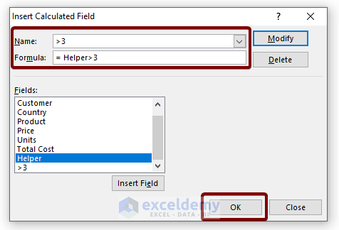
The new column, Sum of >3, now contains 1 for count values of more than 3 and 0 for count values less than 3.

Read More: How to Apply Excel COUNTIF with Pivot Table Calculated Field

Things to Remember

• Convert your data into an Excel Table before converting it again into an Excel Pivot Table.

Download the Practice Workbook

Related Articles

• Pivot Table Calculated Field for Average in Excel
• How to Insert a Calculated Item into Excel Pivot Table
• How to Calculate Variance Using Pivot Table in Excel
• How to Calculate Weighted Average in Excel Pivot Table

<< Go Back to Calculated Field in Pivot Table | Pivot Table in Excel | Learn Excel