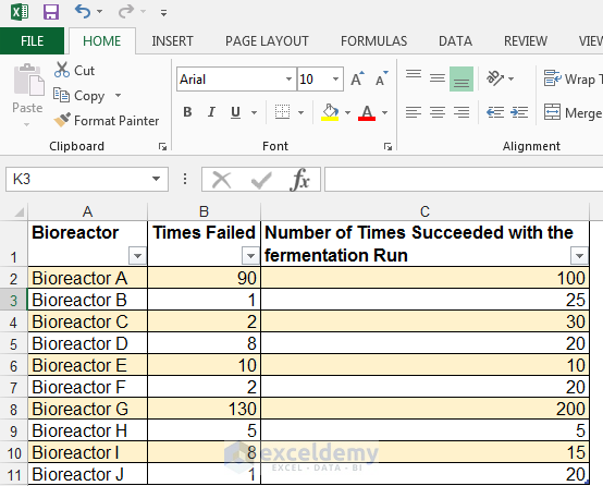
Consider the following: a hypothetical biorefinery has a different bioreactors, producing both biofuel and value-added chemicals. The biorefinery uses microorganisms and fermentation routes. The number of times the equipment failed, and the number of times fermentation succeeded are recorded.
Read More: How to Create Pivot Table Data Model in Excel 2013
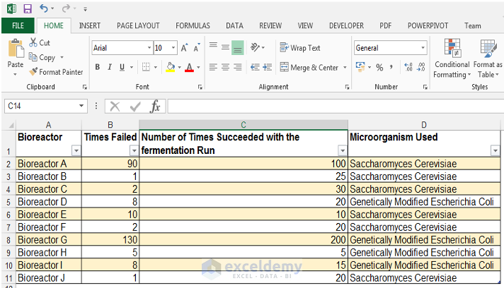
A picture of the source data is shown below:
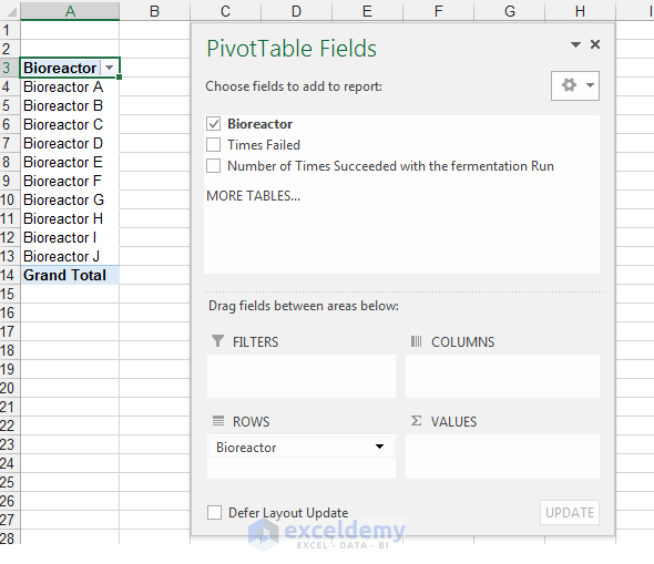
- Create your Pivot Table. (Click the following link: creating pivot tables).
Example 1 – Create a calculated field
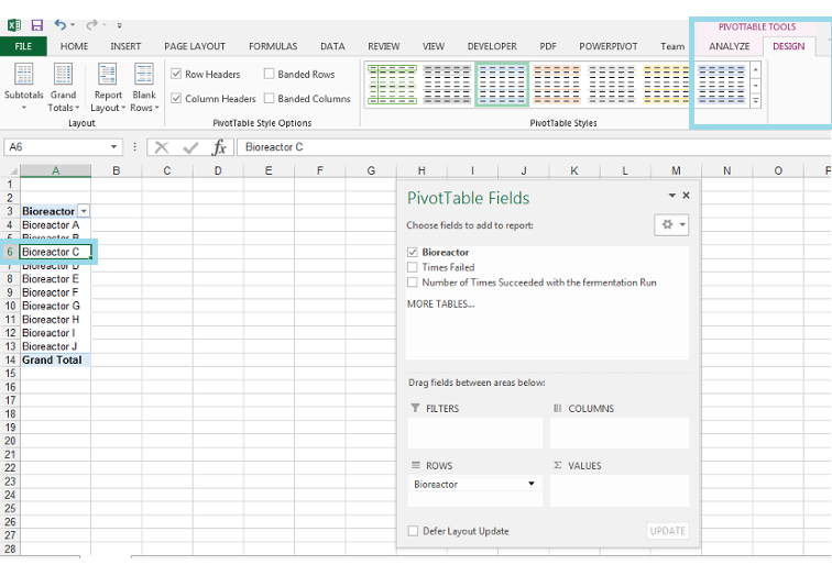
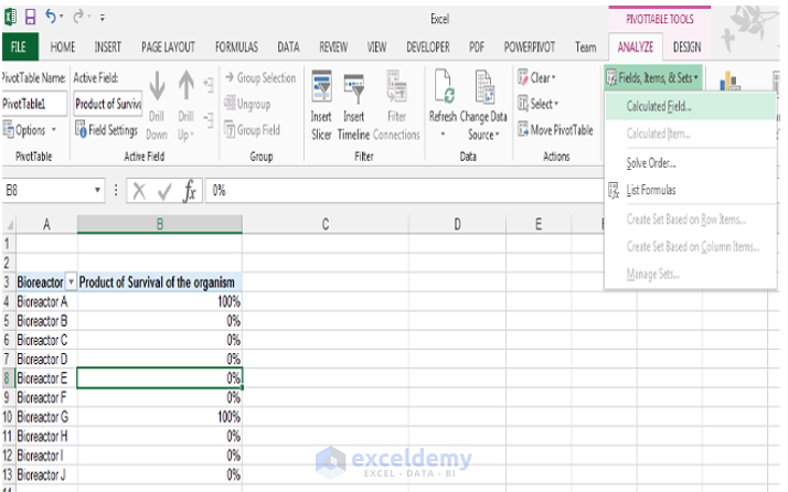
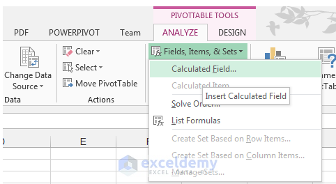
- Select a cell in the Pivot Table to activate Pivot Table Tools, in the Analyze tab.
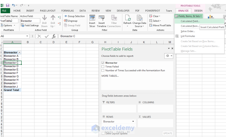
- Click the drop-down arrow next to Fields, Items, & Sets in Calculations.
- Select Calculated Field.
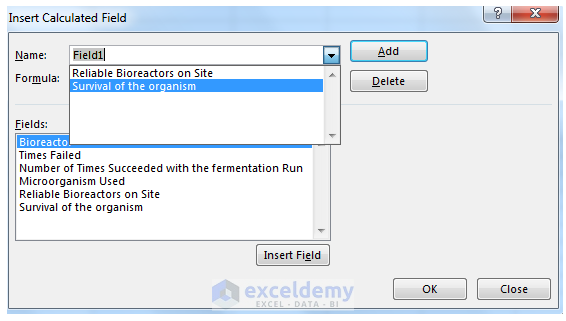
- Choose a name in the Insert Calculated Field dialog box. Here, ‘Reliable Bioreactors on Site’.
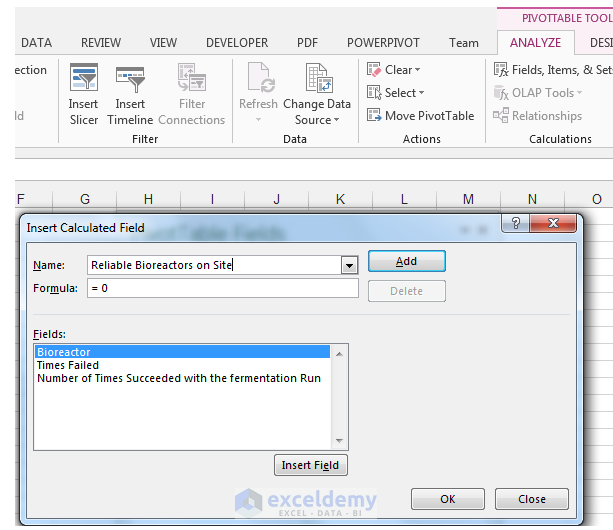
- In the Formula field, enter the formula:
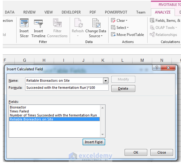
= (‘Times Failed’/ ‘Number of Times Succeeded with the fermentation run’)*100
It will return the failure rate.
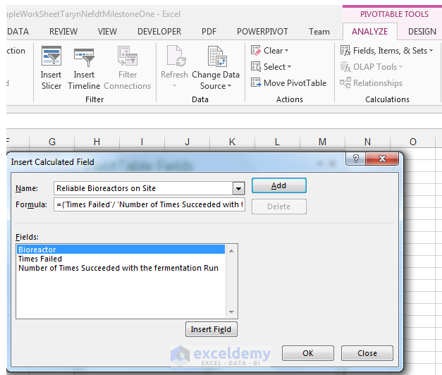
- Click Add to see the new calculated field.
- Click OK.
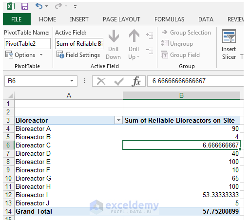
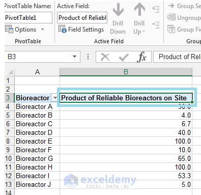
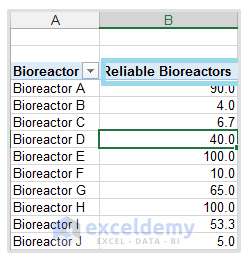
This is the output.
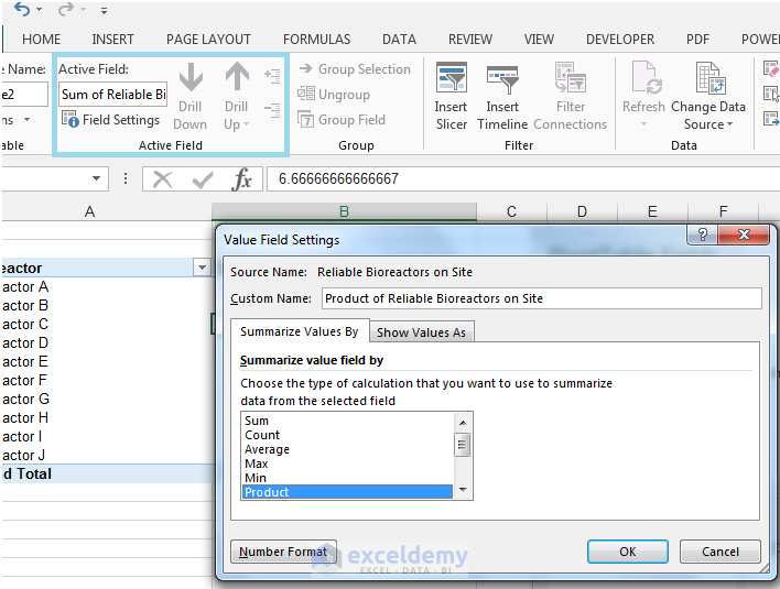
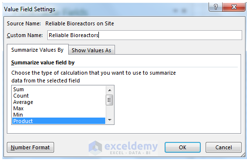
- Go to Field Settings.
- In Value Field Settings, choose Product.
- Click OK.
- Go back to Field Settings.
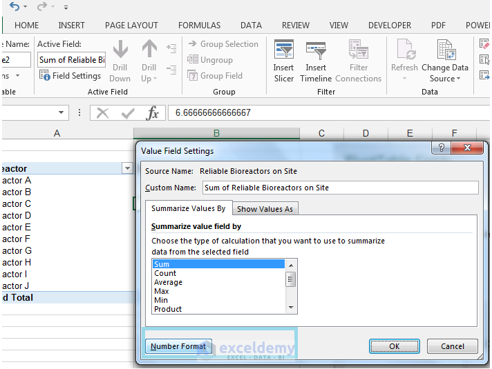
- In the Value Field Settings dialog box, click Number Format.
- Select Number and set the decimal places to 1.
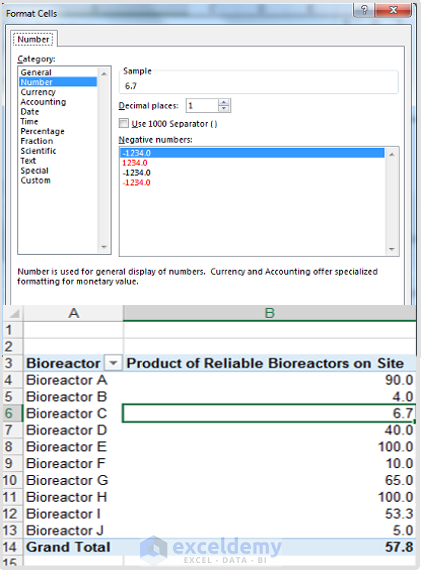
Bioreactors A, H, and E had the highest failure rates.
Example 2 – Create a Calculated Field using the IF Statement
The original dataset was updated: The ‘Microorganism Used’ column was inserted in the source data. Microorganisms are used in the bioreactor to produce biofuel and other products.
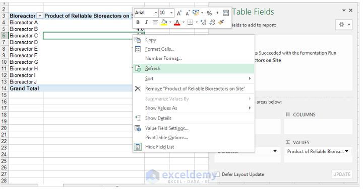
- Select a cell in the Pivot Table and right-click to Refresh, and see the updated fields.
- Create a calculated field to find the number of times fermentation succeeded, irrespective of failure. If it succeeded more than 50 times, the growth of the organism reached the optimum level. If it is less than 50, the organism did not survive in the bioreactor.
Read More: How to Create an Average Calculated Field in Excel Pivot Table
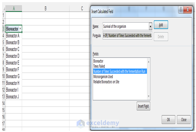
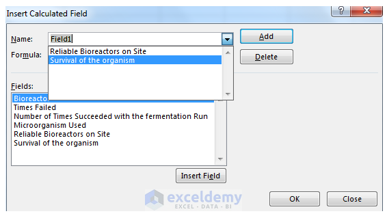
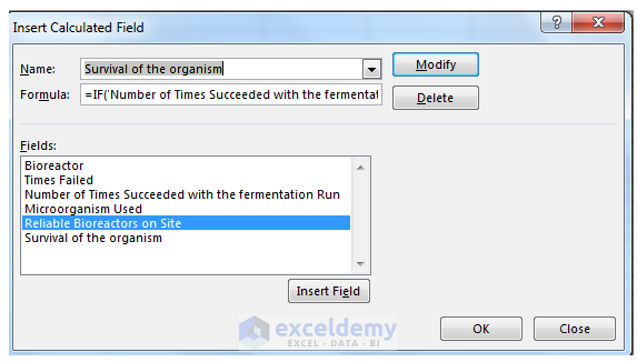
- Name the Calculated Field ‘Survival of the organism’.
- Use the formula below:
= IF( ‘Number of Times Succeeded with the fermentation Run’>=50,100%,0)
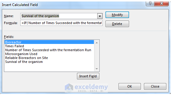
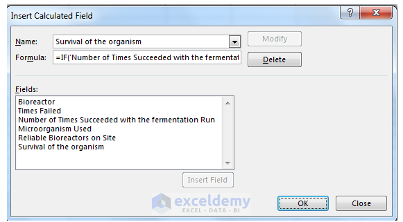
- Click Add.
- Click OK.
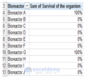
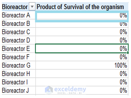
This is the output.
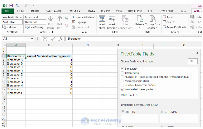
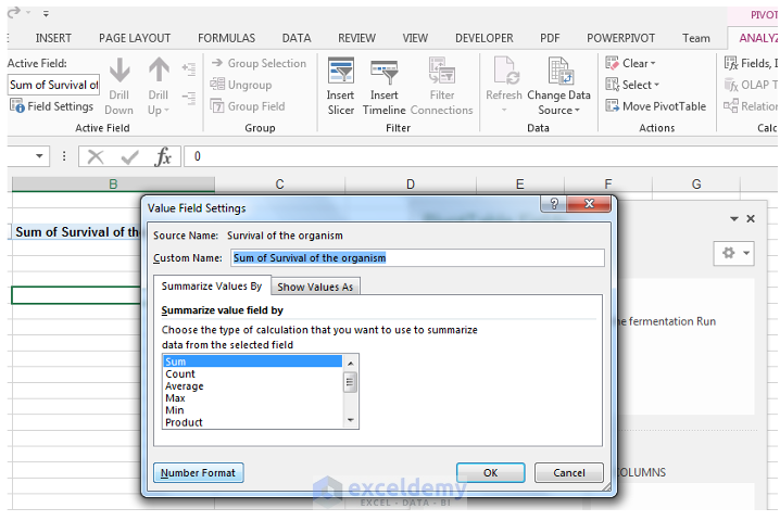
- Go to Field Settings.
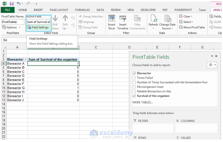
- Choose Number in the Value Field Settings dialog box.
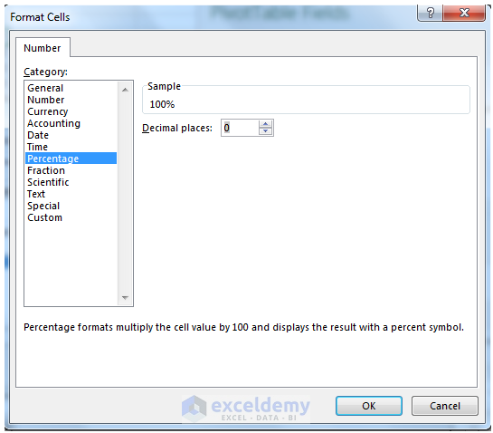
- Click Percentage and choose 0 decimal places.
- Click OK and then OK again to close both dialog boxes.
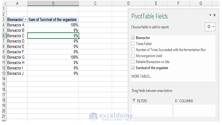
This is the output: even though the bioreactor A was failing, the organism grew.
Read More: Pivot Table Calculated Field for Average in Excel
Problems with the Calculated Field Tools in Excel Pivot Table
If you face problems with Totals in a Calculated Field:
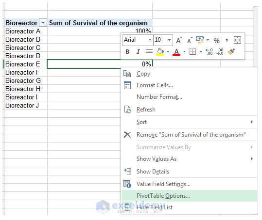
- Right-click a cell in the Pivot Table and Choose PivotTable Options.
- In Totals and Filters tab, uncheck Show grand totals for rows and Show grand totals for columns.
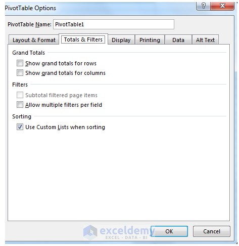
Incorrect Totals are not displayed.
Another common problem is the name of the field.
- In ∑ Values, click the drop-down arrow next to Product of Reliable Bioreactors on Site.
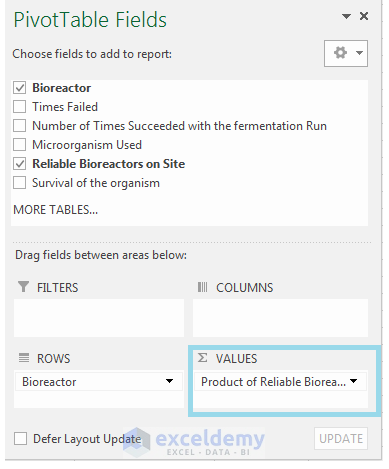
- Go to Value Field Settings…
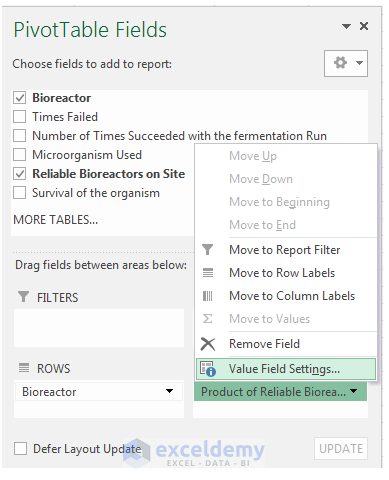
- Change the Custom Name in the Value Field Settings: remove “Product” and enter Reliable Bioreactors.
- Click OK.
How to Edit a Calculated Field?
Read More: Excel Pivot Table Terminology
- Select a cell in the Pivot Table.
- In Calculations, choose Fields, Items & Sets and select Calculated Field.
- Click the drop-down arrow next to Name and select one of the created calculated fields.
- Here, Survival of the organism.
- Adjust the formula, enter:
= IF(‘Number of Times Succeeded with the fermentation Run’ >=105,100%,0)
(50 is changed to 105)
- Click Modify.
- Click OK.
This is the output: Bioreactor A is no longer included in the good growth rate.
How to Delete a Calculated Field in a Pivot Table?
- In the Analyze tab, select Fields, Items & Sets drop-down to display the Calculated Field.
- Click the drop-down arrow next to Name and choose the name of the calculated field you want to delete. Here, Survival of the organism.
- Click Delete.
- Click OK.
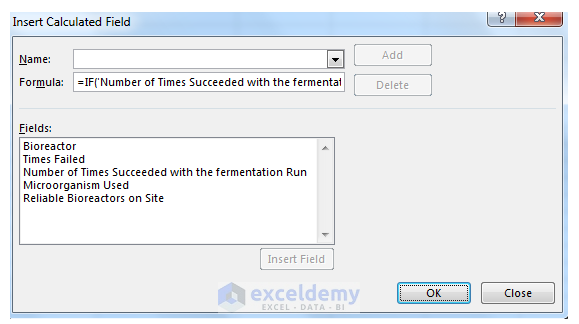
Survival of the organism is deleted both in the Calculated Field and in the Pivot Table Fields List.
Useful Pivot Table related Links from ExcelDemy
How to Use Pivot Table Data in Excel Formulas
8 Excel Pivot Table Examples – How to Make a PivotTable!
Useful links
Excel Pivot Table Tutorials for Dummies Step by Step
Download Working File
Calculated-Fields-Sample-WorkSheet.xlsx
Get FREE Advanced Excel Exercises with Solutions!
