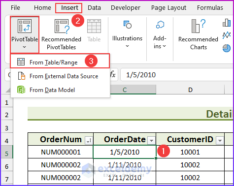
How to Create Pivot Table Data Model in Excel: 6 Methods

Method 1 – Inserting PivotTable

We selected the cell range C5 in the Orders sheet.
From the Insert tab ➪ PivotTable ➪ select From Table/Range.

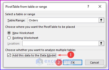
Method 2 – Adding Data to Data Model

A dialog box will pop up.
Select “Add this data to the Data Model”.
Press OK.

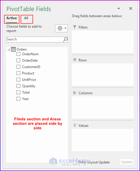
At the PivotTable Fields task pane (on the right side of the newly created worksheet), you will find that it is a bit different as we selected to work with Data Model.
The Task Pane contains two tabs: Active and All. The Active tab lists only the Orders table, and the All tab lists all the tables in the workbook.
Take any table under the All tab to the Active tab. To place the Customers table under the Active tab, activate the All tab, right-click the Customers table, and choose Show in Active Tab from the options. Then do the same for the Regions table.
This is totally optional, later we’ll select the fields from the All tab.
The following figure shows the Active tab of the PivotTable Fields task pane. Customers and Regions tables are expanded to show their column headers (field names). We have also changed the configuration of the task pane (task pane layout). Click on the Tools control, and from the drop-down menu, we choose Fields Section and Areas Section Side-by-Side.

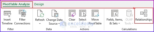
Method 3 – Managing Relationships

Select anywhere inside the new pivot table.
From the PivotTable Analyze tab, select Relationships.

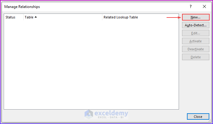
Another dialog box will appear.
Cick New.

Method 4 – Creating Relationship

Another dialog box will pop up.

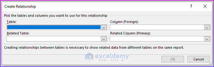
Select the following things:
- Table: Data Model Table: Orders
- Related Table: Worksheet Table: Customers
- Column (Foreign): CustomerID
- Related Column (Primary): CustomerID

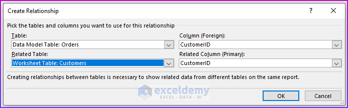
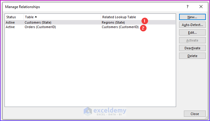
Click OK and you will be returned to the Manage Relationships dialog box.
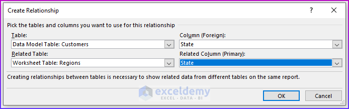
Click New again. Create a relationship between the Customers table and the Regions table, like the following figure.
- Table: Data Model Table: Customers
- Related Table: Worksheet Table: Regions
- Column (Foreign): State
- Related Column (Primary): State
Press OK.

The Manage Relationships dialog box will now show these two relationships.

💡 Notes: If you forget to set up the table relationships in advance, Excel will prompt you to do so when you try to add a field to the pivot table from a different data table.

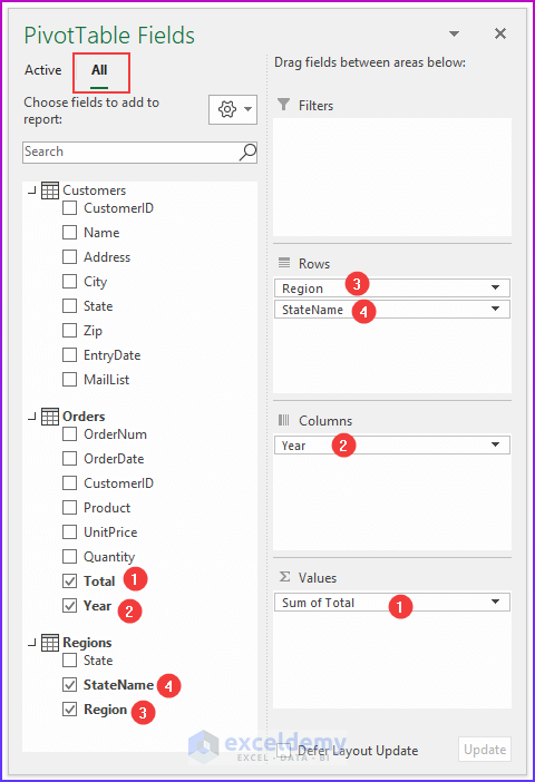
Method 5 – Inserting PivotTable Fields to Areas

Drag the Total field to the Values area.
Move the Year field to the Columns area.
Drag the Region field to the Rows area.
Move the StateName field to the Rows area.

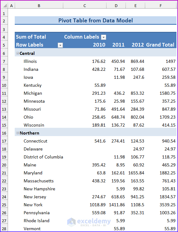
The following figure shows part of the pivot table.

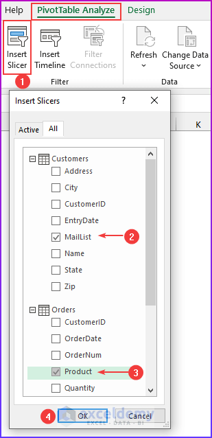
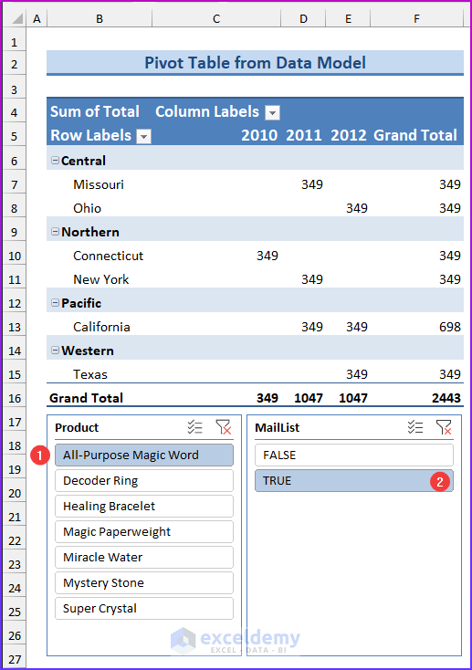
Method 6 – Adding Slicers

Select anywhere inside the pivot table.
Fom the PivotTable Analyze, select Insert Slicers.
From the All tab, select the following things:
- Customers: MaiList.
- Orders: Product.
Press OK.

The final pivot table will look like this.

💡Tips: You can convert the pivot table to formulas. Select any cell in the pivot table and choose PivotTable Tools ➪ Analyze ➪ OLAP Tools ➪ Convert to Formulas. The pivot table will be replaced by cells that use formulas. These formulas are generated with the CUBEMEMBER and CUBEVALUE functions. The new range of data will no longer be a pivot table, the formulas will update when the data changes.

Download Practice Workbook

Creating Pivot Table Data Model.xlsx