Power Pivot is primarily used for managing data tables and the relationships between them, which makes it easier to analyze data from several tables. We can add an Excel table to the Data Model either straight from the PowerPivot Ribbon, or when constructing a PivotTable. In this article, we’ll demonstrate how to add and then remove a Data Model from a Pivot Table.
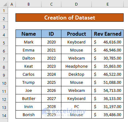
Suppose we have the dataset below, containing information about several Sales representatives. From this dataset, first we will create a data model from the Pivot Table, then we will remove it.
Step 1 – Create Data Model with Proper Parameters
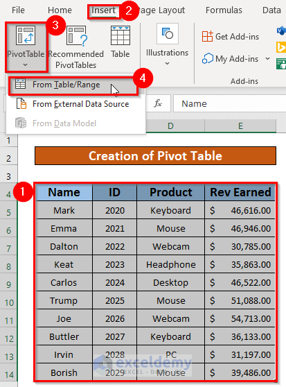
Create a Data Model from the pivot table using our dataset.
- Select the dataset, including the headers (cells B4 to E14).
- From the Insert tab, select Pivot Table.
- Select From Table/Range.
Step 2 – Make Data Model from Pivot Table
The PivotTable from table or range dialog box appears.
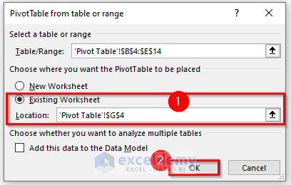
- Check Existing Worksheet.
- Enter ‘Pivot Table’!$G$4 in the Location box.
- Click OK.
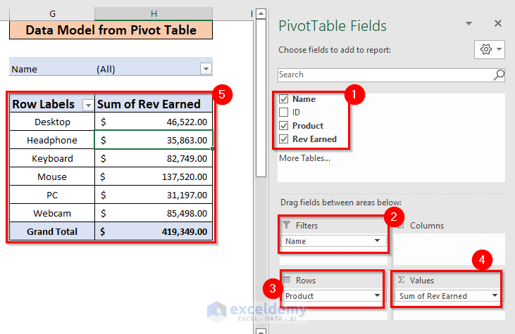
The Data Model from Pivot Table is created.
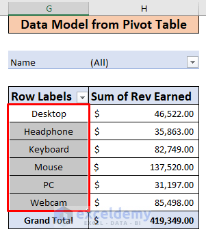
Step 3 – Remove Data Model from Pivot Table
- Select the range G6 to G11.
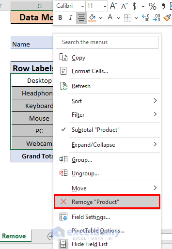
- Place your cursor on the chart and right-click the mouse.
- Select Remove “Product” from the context menu.
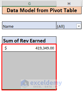
- The Data Model is removed from the Pivot Table.
Things to Remember
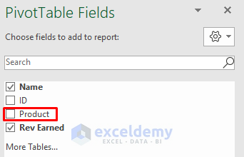
- You can also remove the data model from the Pivot Table itself. Simply uncheck the Product option from the PivotTable Fields.
- When a value can not be found in the referenced cell, the #N/A! error is returned.
- A #DIV/0! error will appear if a value is divided by zero (0) or the cell reference is blank.
Download Practice Workbook
<< Go Back to Pivot Table Data Model | Pivot Table in Excel | Learn Excel
Get FREE Advanced Excel Exercises with Solutions!
