How to Create a Data Model in Excel – 3 Methods

Method 1- Using the Relationships Tool to Create a Data Model in Excel

Steps:

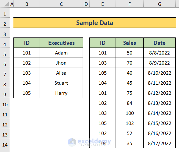
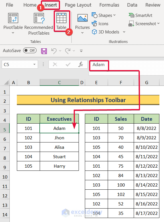
• Select a value in the dataset.
• Go to the Insert tab.
• Select Table.

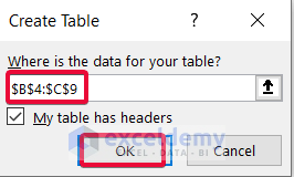
• In Create Table, select the entire dataset as table data.
• Click OK.

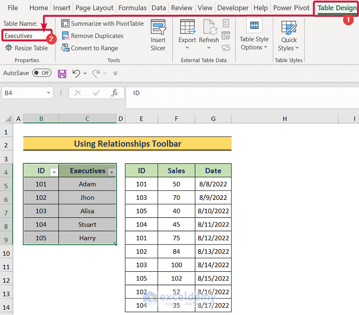
• Go to Table Design.
• Name the created table.
• Repeat the process for the rest of the dataset.

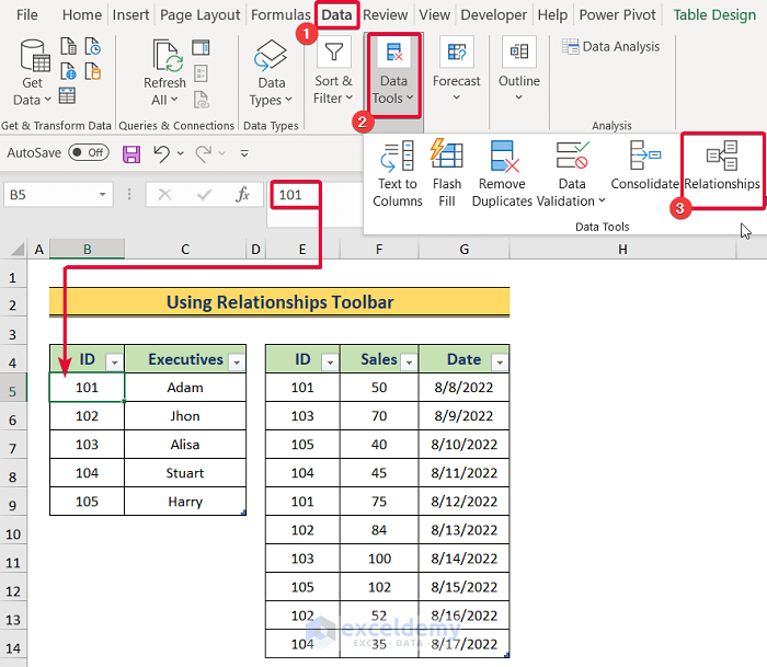
• Go to the Data tab.
• In Data Tools, select Relationships.

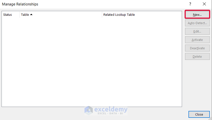
• In Manage Relationships, select New.
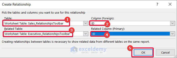
• The Create Relationship prompt will be displayed.

• Select the table you want to analyze. Here, Sales.
• Select the column that is common to both tables as Column(Foreign). Here, ID. It may contain duplicates.
• Select the look-up table as Related Table. Here, Executives.
• Select the common column as Related Column(Primary). Here, ID. It must contain unique values.
• Click OK.

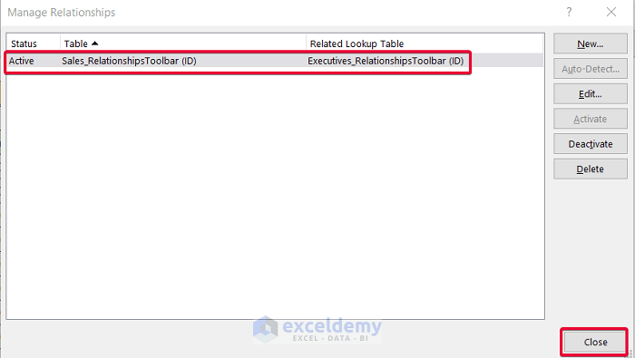
A window displays the relationship.

• Click OK.

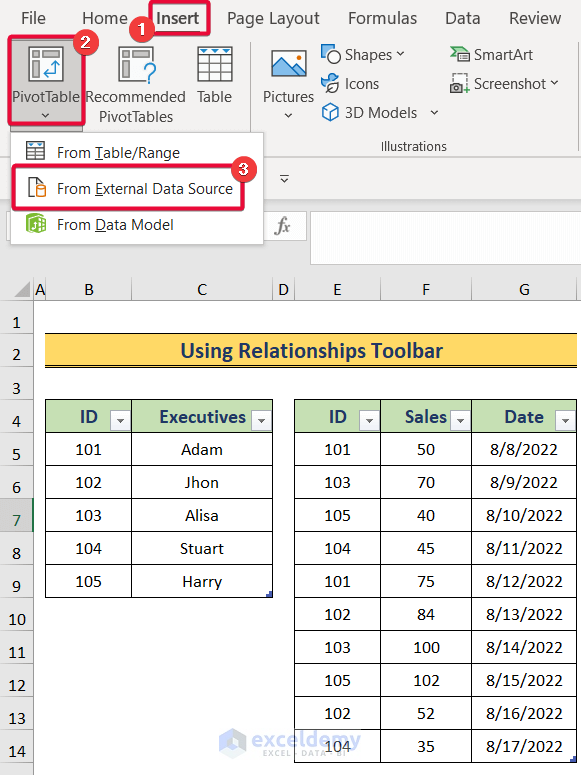
• Go to the Insert tab.
• Click PivotTable.
• Select From External Data Source.

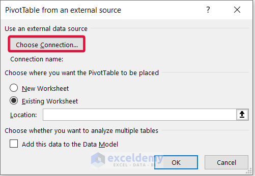
• In the PivotTable from an external source window, select Choose Connection.

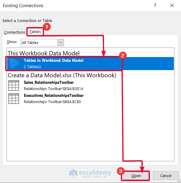
• In the Existing Connections window, go to Tables.
• Excel has listed the two previously connected tables in the Relationships toolbar.
• Choose Tables in Workbook Data Model.
• Click Open.

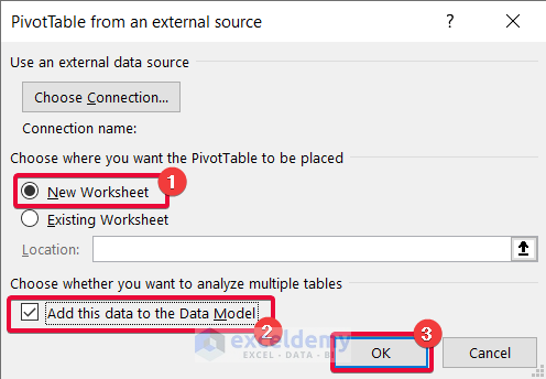
• In the PivotTable from an external source window select New Worksheet.
• Check Add this to the Data Model.
• Click OK.

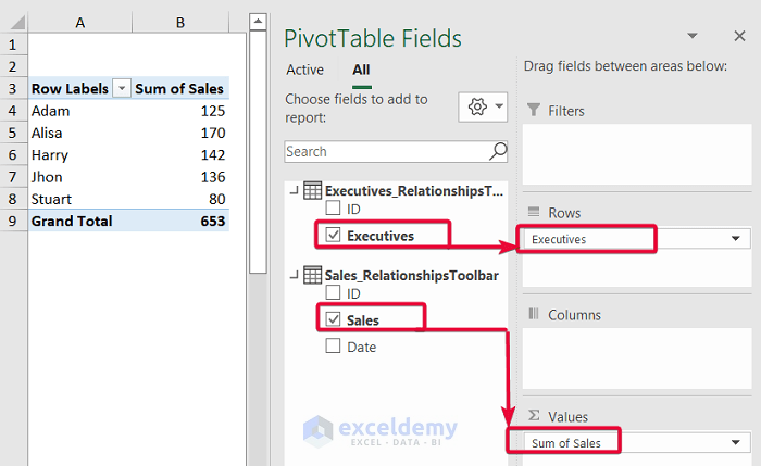
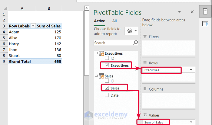
A pivot table is created using the data model. Here, you can relate the two tables:  you can select the executives’ names in the Executive table and find their sales numbers in the Sales table.

Read More: How to Get Data from Data Model in Excel

Method 2 – Creating a Data Model with the Excel Power Query

Steps:

• Select a value in the dataset.
• In Insert, select Table.

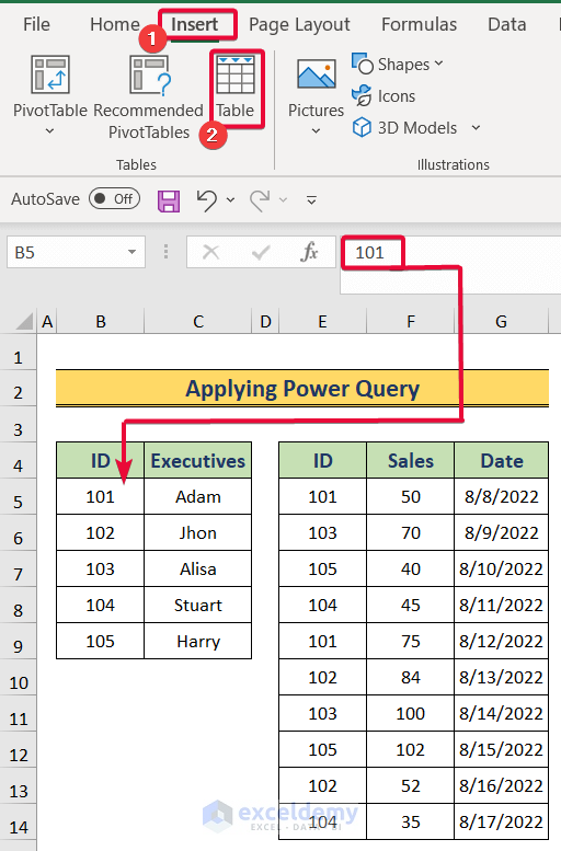
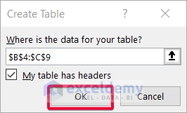
• Select the entire dataset as table data in Create Table.
• Click OK.

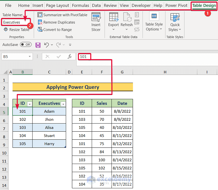
• Select Table Design and name the created table.
• Repeat the process for the other datasets.

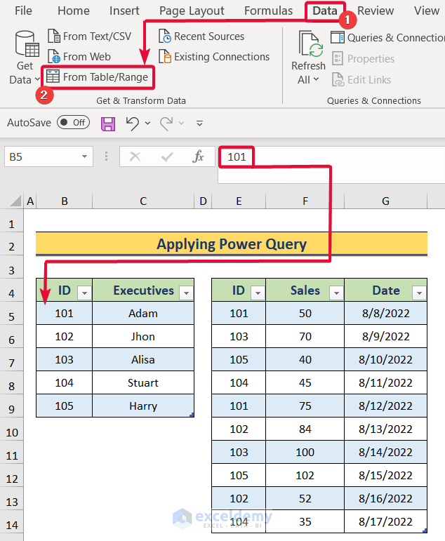
• Go to the Data tab and select From Table/Range.
• The Power Query window will be displayed.

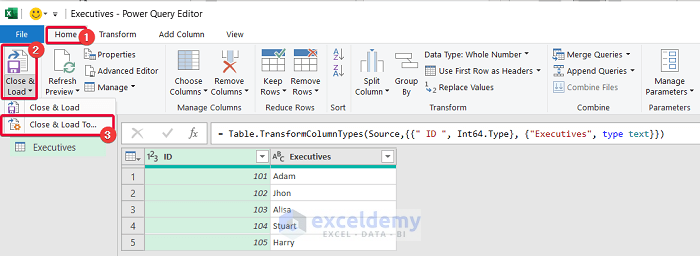
• In the Power Query Editor, select the Home tab.
• Choose Close & Load.
• Select Close & Load To… .
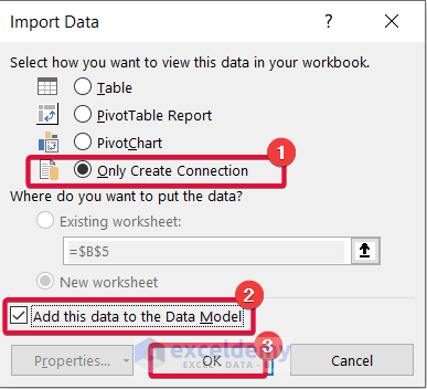
• The Import Data window will be displayed.

• Choose Only Create Connection and check Add this to the Data Model.
• Click OK.
• Repeat this process for the rest of the tables.

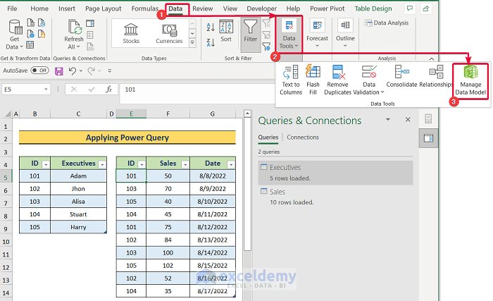
• Go to the Data tab and choose Data Tools.
• Select  Manage Data Model.

• In the new window, select the Home option.
• Select View and choose Diagram View.

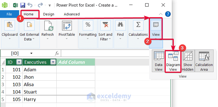
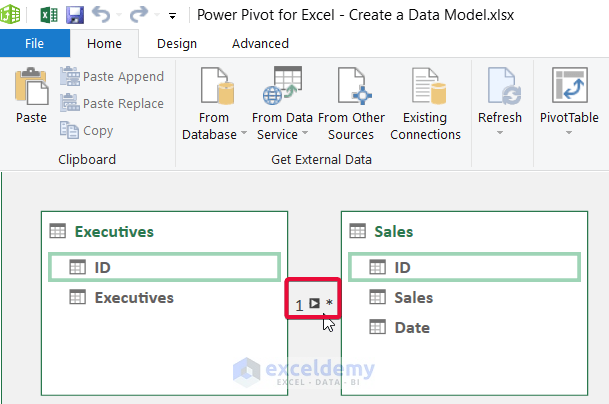
You will see the tables as diagrams.

• Connect the common columns of the two tables. Here, ID.
• The connection displays 1 on one side and an asterisk on the other: the tables have a One to Many relationship. 1 means that the Executive ID column has no duplicate values. On the other hand, the  ID column in the Sales table has duplicate values.

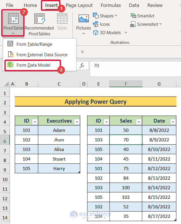
• Go to the Insert tab.
• Select PivotTable.
• Select From Data Model.

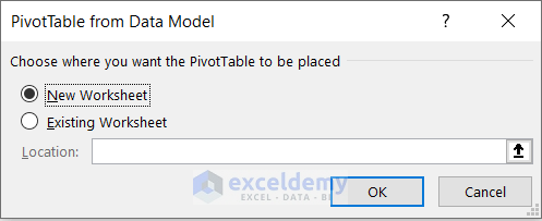
• Select New Worksheet.
• Click OK.

The data model was used to create a pivot table: you can relate the two tables. For example, choose the names of the executives in the Executives table and look up their sales numbers in the Sales table.

Read More: Excel Data Model vs. Power Query: Main Dissimilarities to Know

Method 3 – Applying a Power Pivot to Make a Data Model in Excel

Steps:

• Select a cell in the dataset.
• Go to the Insert tab and choose Table.

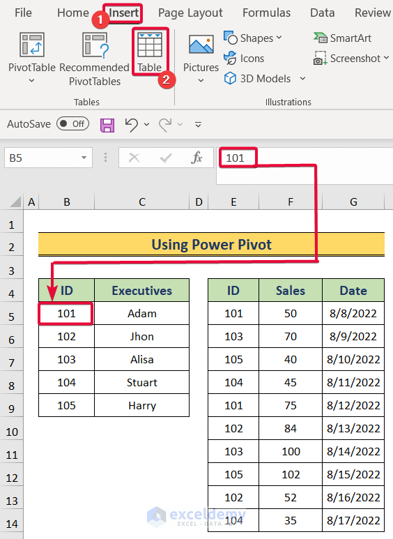
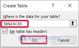
• In Create Table, select the entire dataset.
• Click OK.

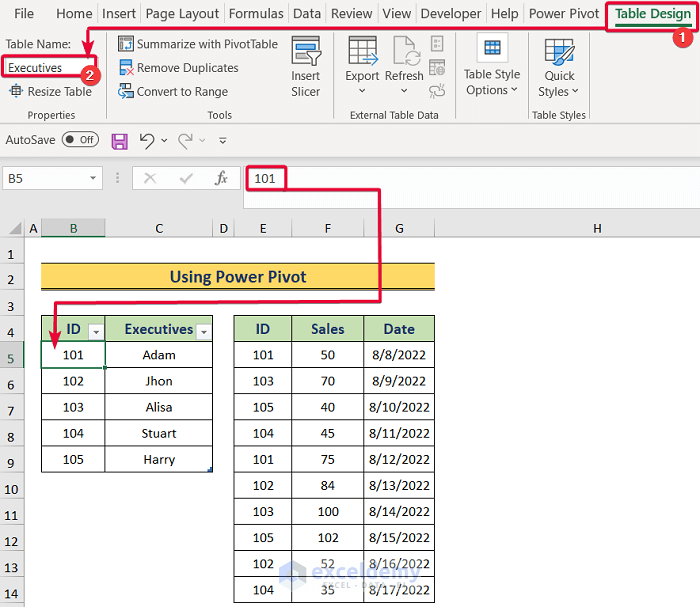
• Go to Table Design and name the created table.
• Repeat the process to create other tables.

• Go to the Power Pivot tab and select Add to Data Model.

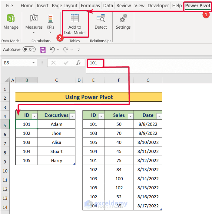
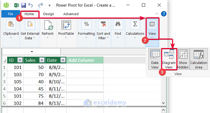
• In the Power Pivot window, go to the Home tab.
• In View, select Diagram View.

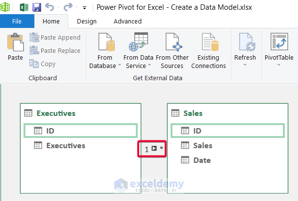
• Connect the two common columns from the two table diagrams. Here, ID.

The two tables are connected in a One to Many relationship.

• Go to the Home tab and choose PivotTable.

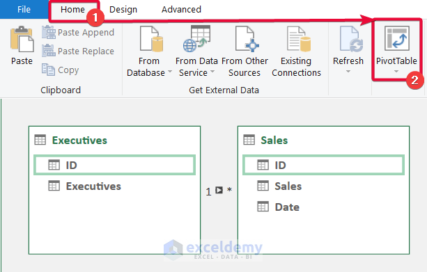
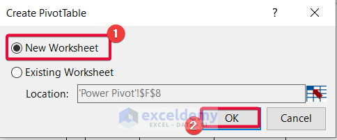
• In Create PivotTable, select New Worksheet.
• Click OK.

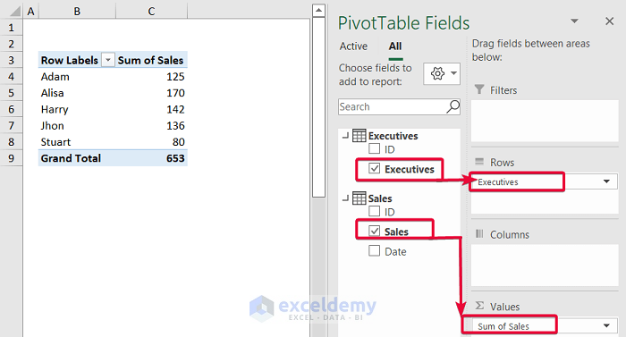
• A pivot table with two tables will be displayed.
• A data model relates the two tables.

Read More: How to Add Table to Data Model in Excel

Download Practice Workbook

Related Articles

• How to Update Data Model in Excel
• How to Use Reference of Data Model in Excel Formula
• How to Remove Table from Data Model in Excel

<< Go Back to Data Model in Excel | Learn Excel