When working with an interlinked, large, and complex dataset in Excel, creating data models is a great approach to solving multiple calculations easily. Now, there might be some updates to those data models at times. In this article, I will show you 2 suitable ways to update the data model in Excel.
What Is Data Model in Excel?
A data model is a special type of table where multiple tables can be correlated. In this type of table, you can connect two or more tables with single or multiple columns. When working with large, interlinked data, this table is a blessing.
Suppose, you have two different tables; one containing the student Ids, students’ names, and genders, the other containing marks of different subjects with only student Ids. Now, you can interlink them within a data model, and thus, you will get every student’s Ids, names, genders, and marks in different subjects altogether.
How to Update Data Model in Excel: 2 Suitable Ways
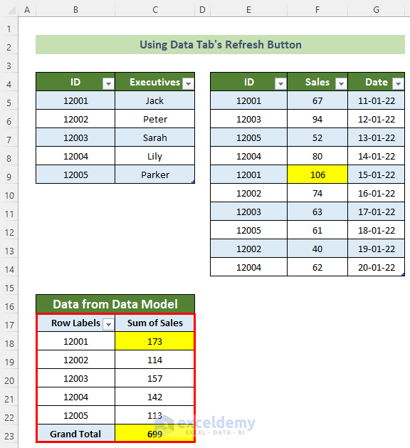
Say, you have a dataset primarily with 2 ranges. One is containing IDs and Executive’s names. The other one contains Ids, Sales and Dates.
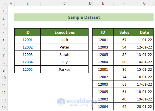
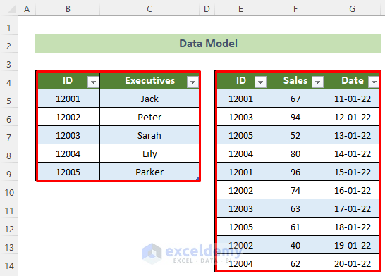
Now, from these ranges, you have created a data model primarily.
Now, you need to update this data model if any change happens or if any additional row or column needs to be added. Follow the 2 suitable ways below to update data model in Excel.
1. Use Refresh Button of Data Tab
From data models, we extract results through Pivot Table easily. Now, say, you have changed data inside the data model’s table. But you need to update the data model properly for getting the updated result in the pivot table. Follow the steps below to accomplish this.
📌 Steps:
- First, you need to get data from the data model.
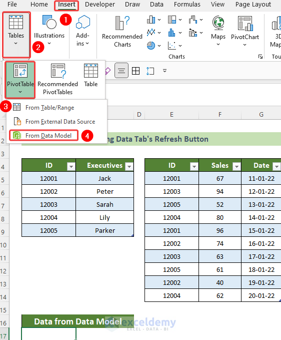
- To do this, click on a cell (B17 here) where you want the pivot table.
- Afterward, go to the Insert tab >> Tables group >> PivotTable tool >> From Data Model option.
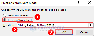
- As a result, the PivotTable from Data Model window would appear.
- Following, put the radio button on the Existing Worksheet option >> choose your desired location of pivot table in the Location: text box >> click on the OK button.
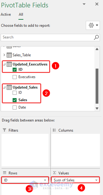
- Afterward, a pivot table would appear in cell B17 and a pane named PivotTable Fields would appear on the right side.
- Here, your tables’ names in this worksheet are Updated_Executives and Updated_Sales.
- Following, tick on the field ID from the Updated_Exceutives table and Sales field from the Updated_Sales table.
- Subsequently, put the ID field on the Rows group below and the Sum of Sales field on the Values group.
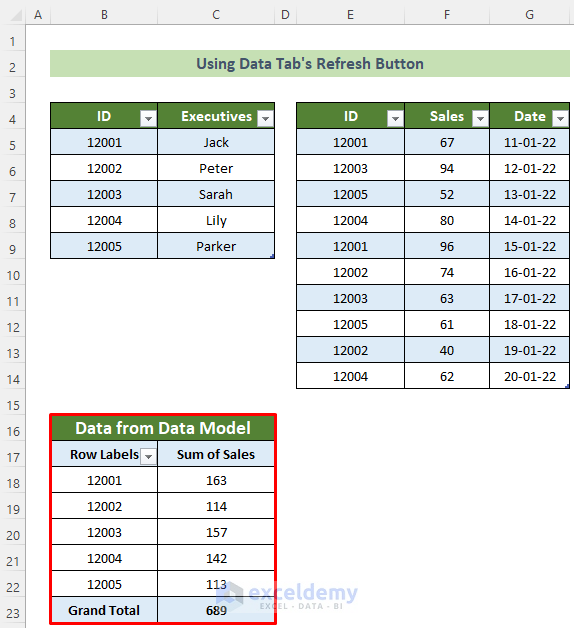
- Thus, you would see there would be a Pivot table with IDs and Sales on cell B17.
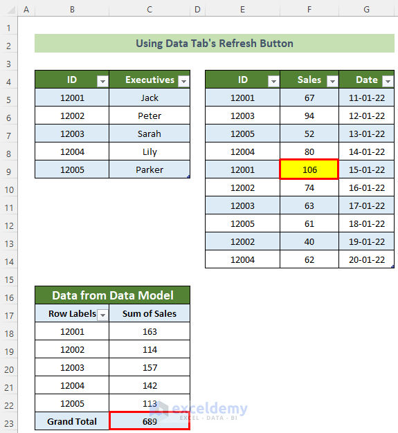
- Now, say, you have changed data on cell F9 of your Updated_Sales table of this data model.
- But, you can see the pivot table is not showing the exact results yet. So, the data model is not updated properly.
- Now, go to the Data tab >> Refresh All button >> Refresh All option.
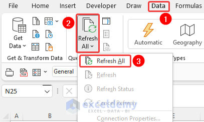
- Consequently, you will see your data model has been updated properly now and the pivot table is showing exact results.
Thus, you have successfully updated your data model in Excel. And, the outcome would look like this.
Read More: How to Use Data Model in Excel
2. Using Power Pivot to Update Data Model in Excel
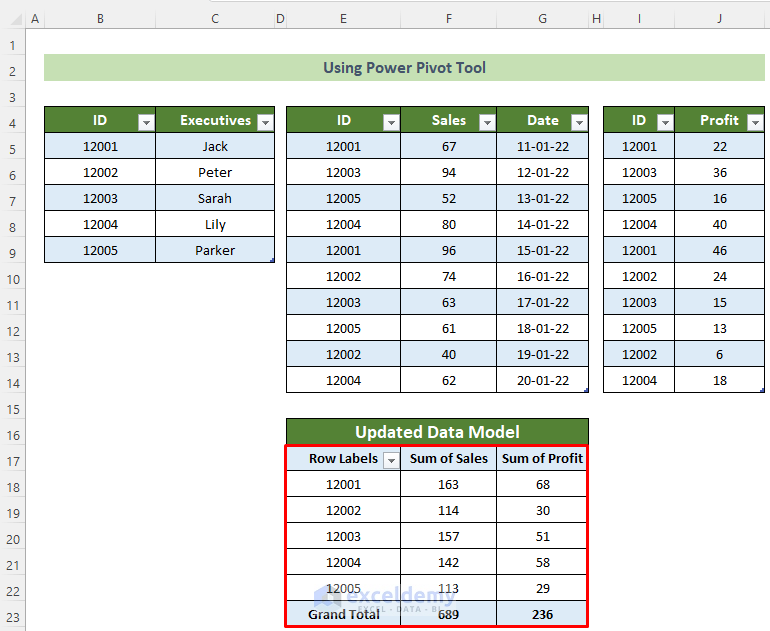
Now, say you have an extra range to add to your data model. This range contains two columns named ID and Profit.
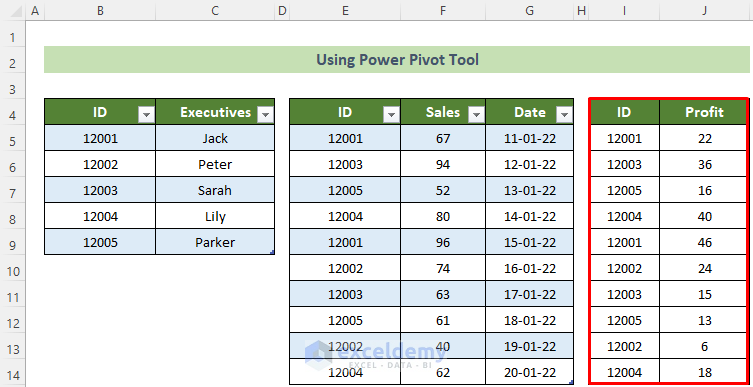
Now, you can add this range to the data model and get the updated results by following the steps below.
📌 Steps:
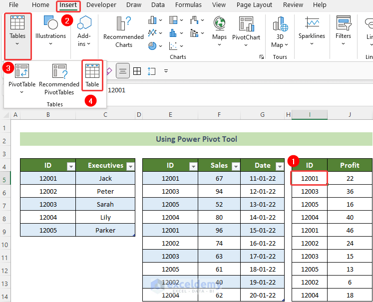
- First, you need to insert this range as a table.
- To do this, click anywhere inside the range (cell I5 here) >> go to the Insert tab >> Tables group >> Table tool.
- As a result, the Create Table window will appear.
- Here, declare your data range inside the first text box >> tick on the option My table has headers and click on the OK button.
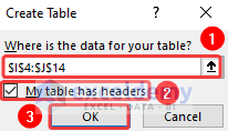
- Consequently, you will be able to convert the range into table.
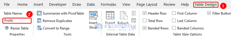
- Now, go to the Table Design tab >> name the table as Profit in the Table Name: text box.
- Afterward, click on any cell (I5 here) inside the new table >> go to the Power Pivot tab >> Add to Data Model tool.
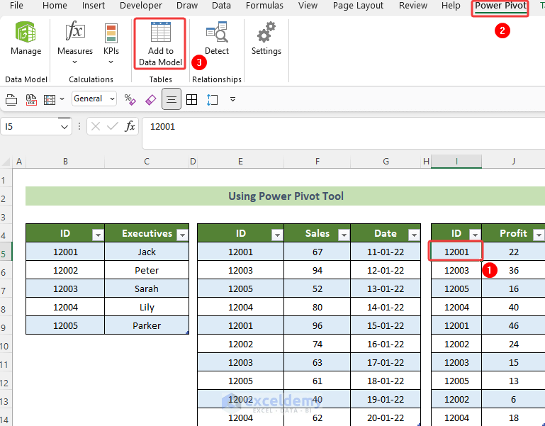
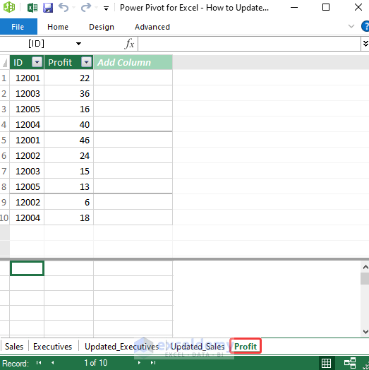
- As a result, the Power Pivot from Excel window would appear and show you that the Profit table is added into the data model.
- Now, repeat the steps 1 to 6 from the first method described above to insert a pivot table into the Excel with data model results.
- Now, here, the tables of Executives and Sales are named as Executives_Table and Sales_table.
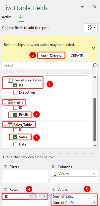
- So, focus on the PivotTable Fields pane on the right side of Excel.
- Here, tick on the value ID from the Executives_Table table, tick on the value Profit from the Profit table, and tick on the value Sales from the Sales_Table table.
- Following, drag the ID value on the Row group and keep the Sum of Sales value and Sum of Profit value on the Values group.
- Last but not least, there would be a warning about the new relationships between tables is needed.
- Subsequently, click on the Auto-Detect… button. Or, you can manually create relationships between tables by clicking on the CREATE… button.
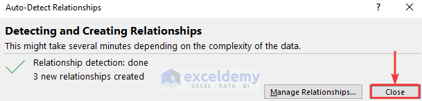
- Consequently, the pivot table will be created on the selected cell and there will be a window named Auto-Detect Relationships where you will be informed about the auto created relationships.
- Subsequently, click on the Close button.
Finally, you would get the pivot table results as an update to your previous data model and with extra tables added into the data model. And, the final outcome should look like this.
Read More: Excel Data Model vs. Power Query: Main Dissimilarities to Know
💬 Things to Remember
You must create relationships between tables in your data model. Otherwise, you won’t get accurate results up to your requirements.
Download Practice Workbook
You can download our practice workbook from here for free!
Conclusion
So, in this article, I have shown you 2 suitable ways to update a data model in Excel. You can also download our free workbook to practice. I hope you find this article helpful and informative. If you have any further queries or recommendations, please feel free to comment here. Have a nice day! Thank you!
Related Articles
- How to Remove Table from Data Model in Excel
- How to Use Reference of Data Model in Excel Formula
- How to Add Table to Data Model in Excel
<< Go Back to Data Model in Excel | Learn Excel
Get FREE Advanced Excel Exercises with Solutions!
