How to Create Calculated Field in Pivot Table Data Model: 4 Methods

Method 1 – Creating Implicit Calculated Field in Pivot Table Data Model

Step-01: Creating Pivot Table

• Go to the Insert tab >> PivotTable dropdown >> From Table/Range option

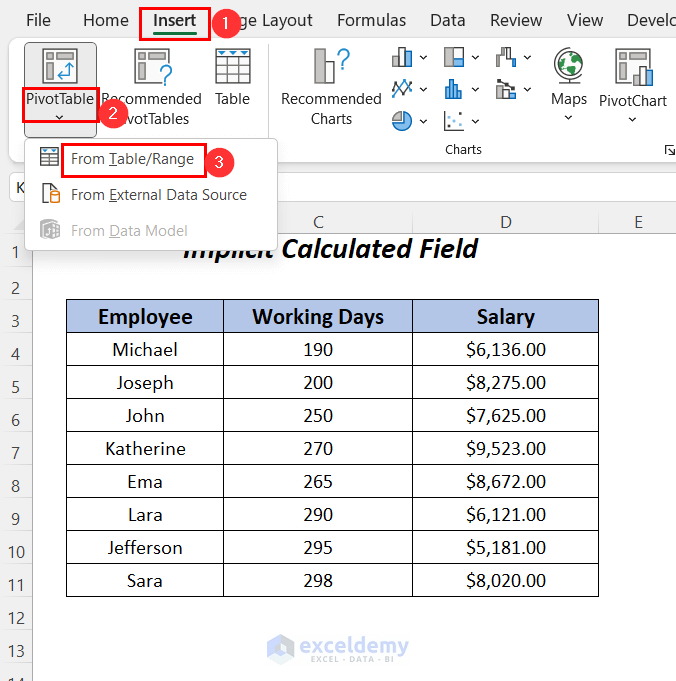
The PivotTable from table or range dialog box will appear.

• Select the dataset as Table/Range, and click on the New Worksheet
• Check the Add this data to the Data Model option and press OK.

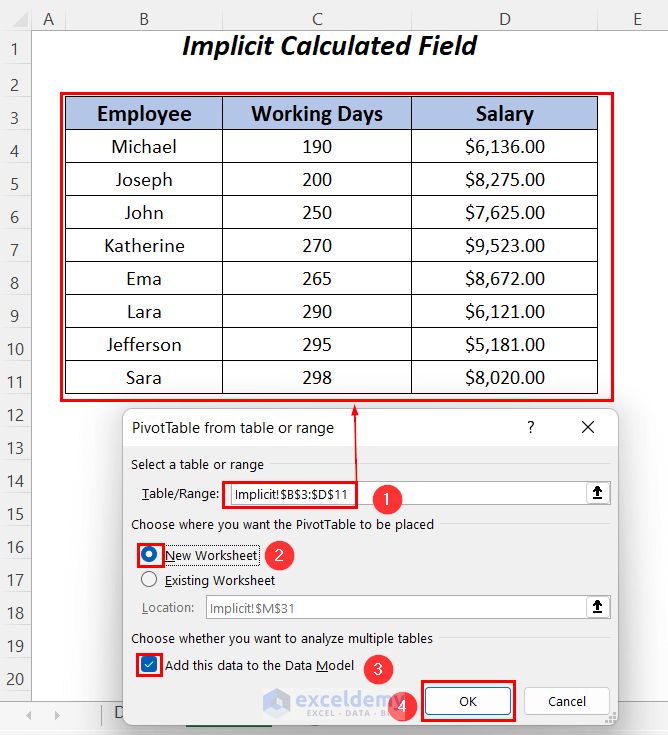
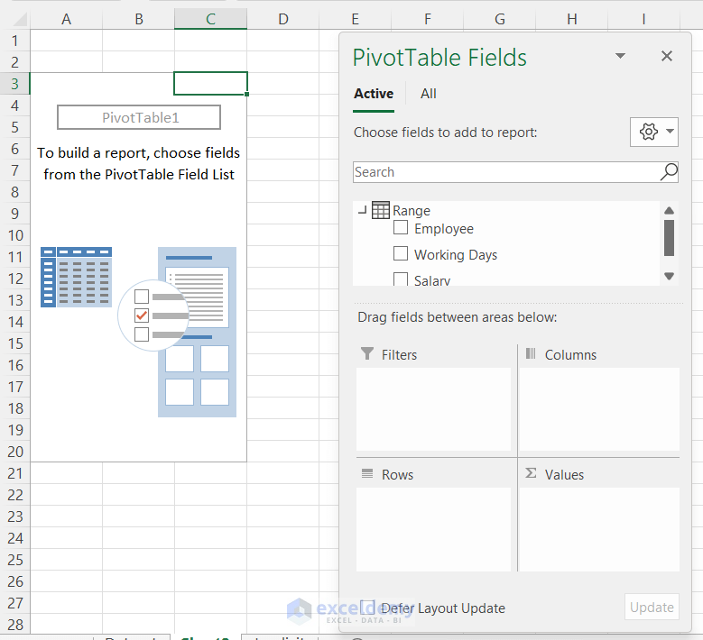
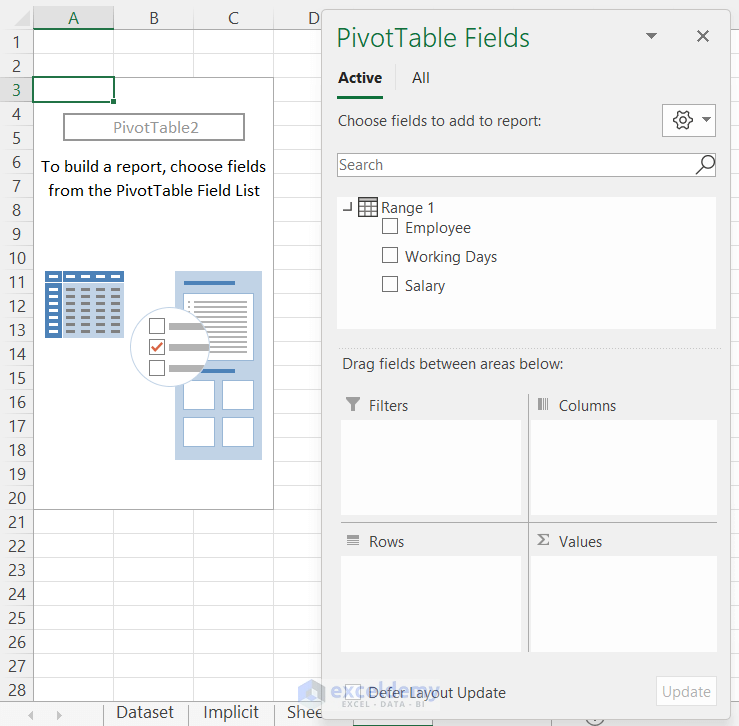
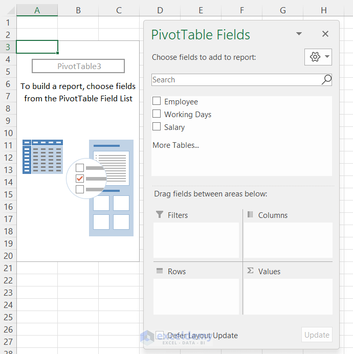
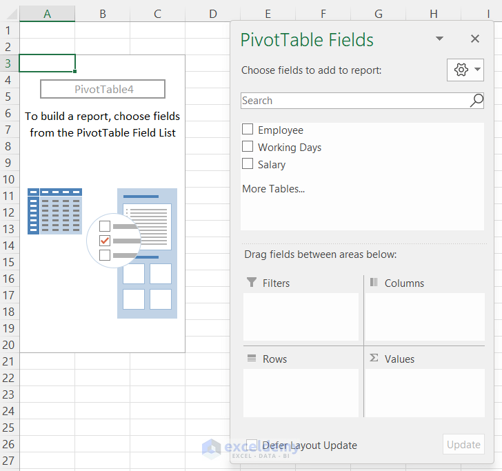
You will go to a new sheet containing two portions; PivotTable1, and PivotTable Fields.

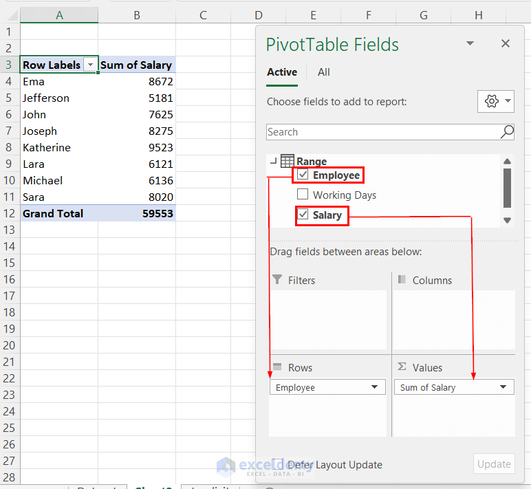
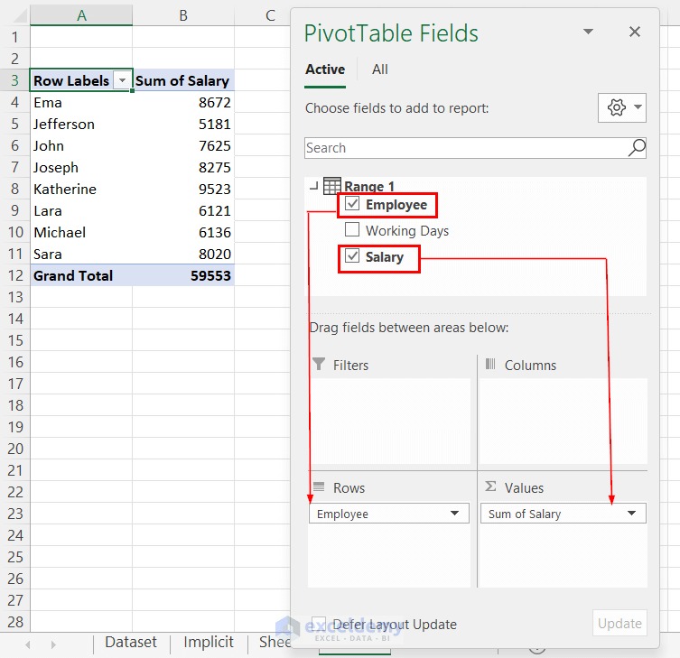
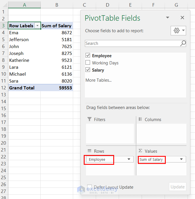
• Drag down Employee to the Rows area and Salary to the Values

The following PivotTable will appear on the left side.

Step-02: Adding Measure to Enter Calculated Field

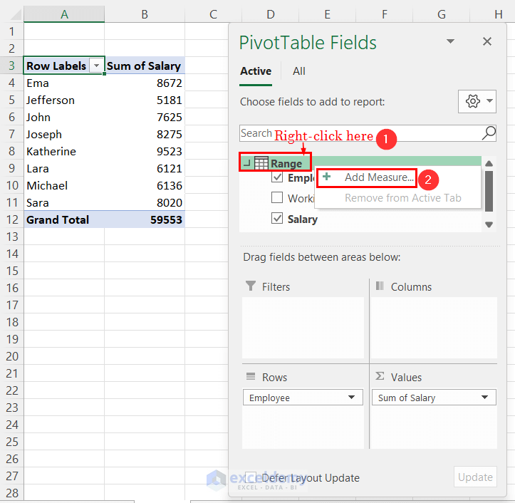
• Right-click on the name of the PivotTable (here, it is Range)
• Choose the Add Measure…

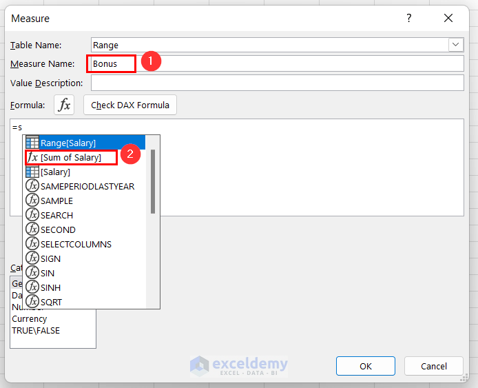
The Measure dialog box will pop up.

• Type Bonus (or whatever you want) in the Measure Name.
• In the Formula box after the equal (=) sign type your formula. You want the Sum of Salary field and so after typing s, you will see various options. You will select the [Sum of Salary].

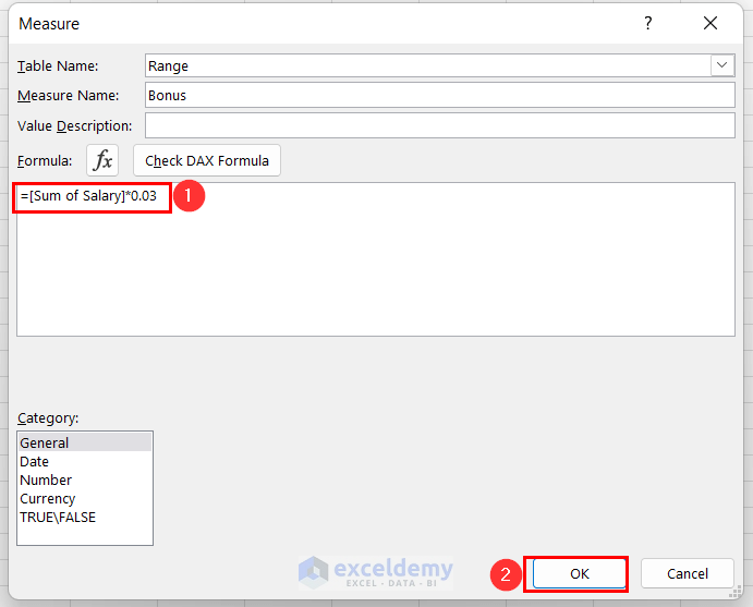
• Write down the complete formula

We multiplied 0.03 with [Sum of Salary] because the bonus will be 30% of an individual’s salary.

• Press OK.

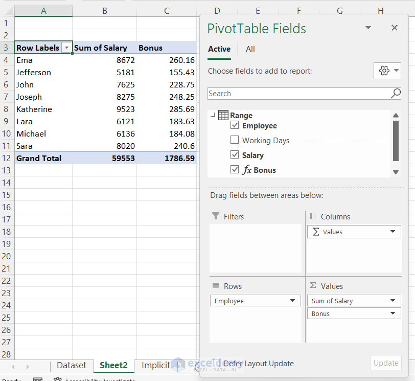
Our calculated field Bonus will appear in the field list.

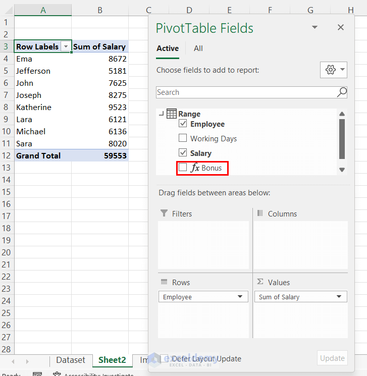
• Drag down the Bonus field to the Values.

The new column Bonus will appear with the calculated values.

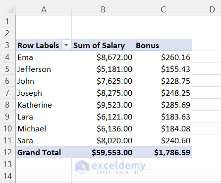
After adding the currency symbols to the salaries and bonuses, you will have the following figure.

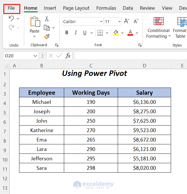
Method 2 – Creating Implicit Calculated Field with Power Pivot Tab

Step-01: Enabling Power Pivot Option

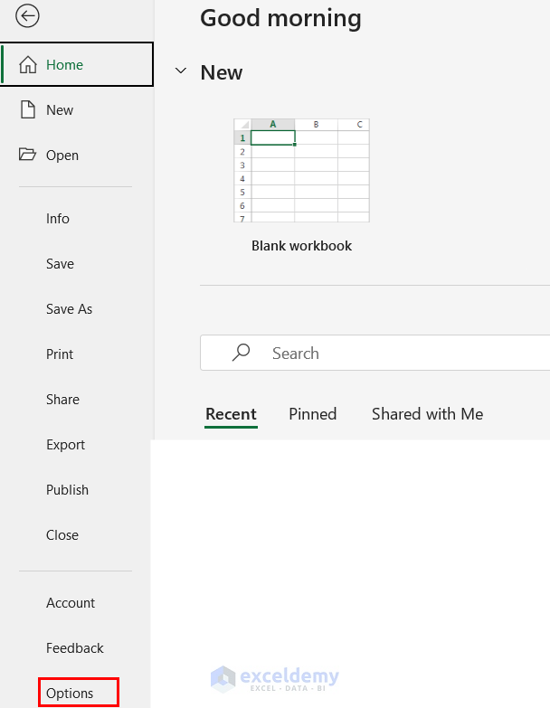
• Go to the File tab.

• Select Options.

You will have the Excel Options wizard.

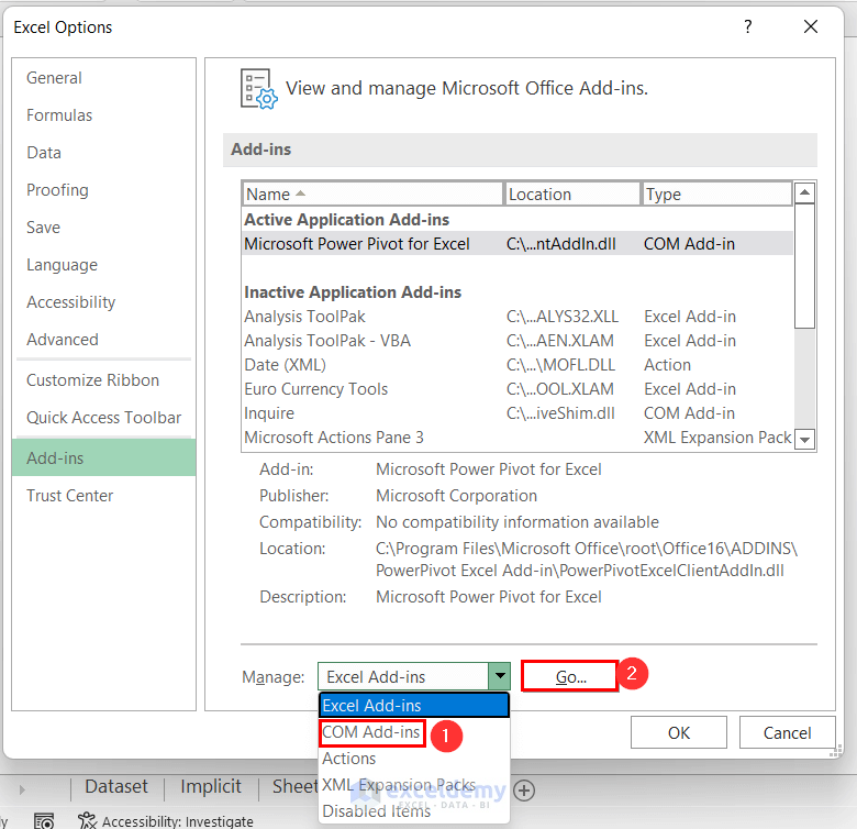
• Go to the Add-ins tab and click on the dropdown symbol beside the Manage.

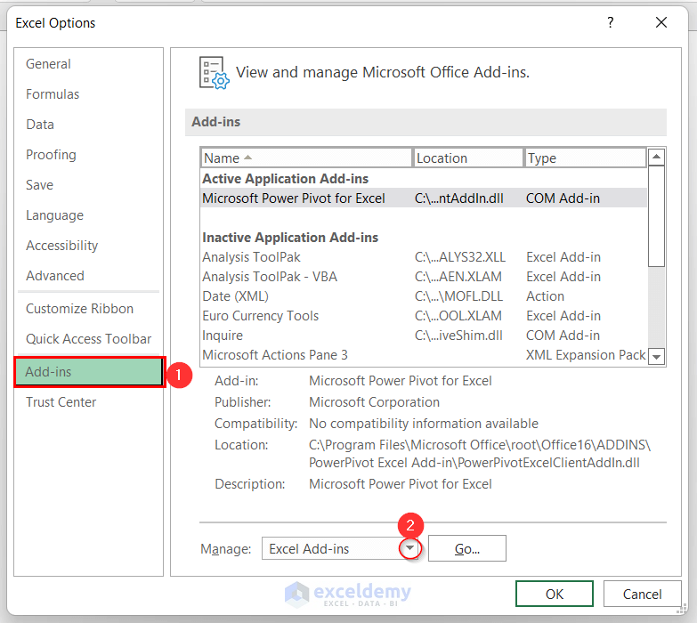
• Choose the COM Add-ins option and click Go.

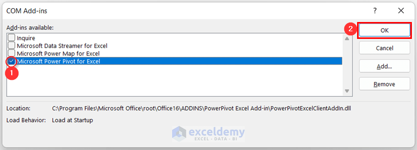
The COM Add-ins wizard will open up.

• Check the Microsoft Power Pivot for Excel option and press OK.

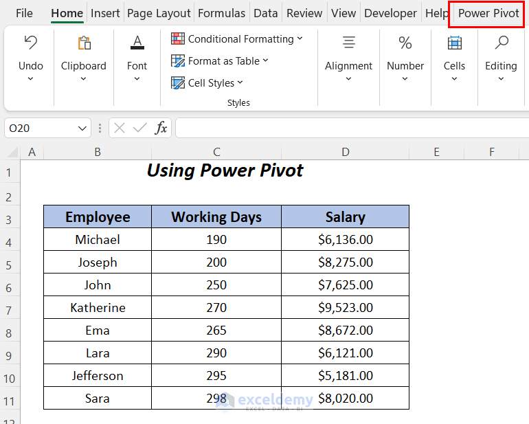
You will see the Power Pivot tab in your workbook.

Step-02: Adding Measure to Enter Calculated Field

• Follow Step-01 of Example-1 to open up the following sheet.

• Drag down Employee to the Rows area and Salary to the Values.

The following PivotTable will appear on the left side.

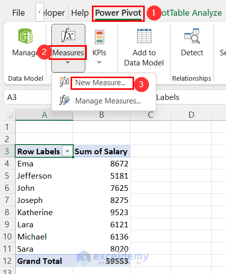
• After selecting any cell of your PivotTable, go to the Power Pivot tab >> Measures dropdown >> New Measure

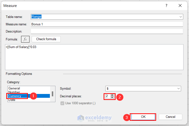
You will have the Measure dialog box.

• Set the Measure name as Bonus 1.
• Write down the following formula in the Formula box.

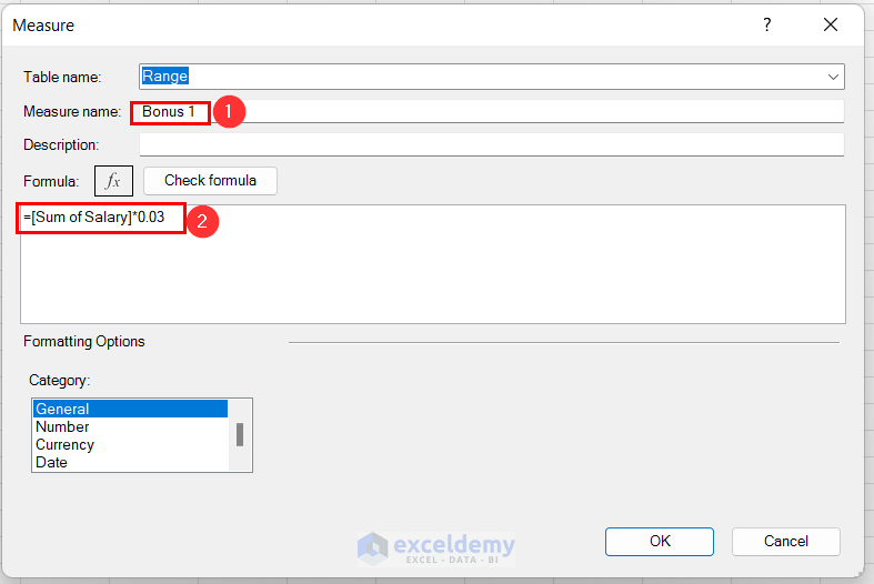
You can change the formatting here.

• Choose Currency as Category and keep the Decimal places up to 2.
• Press OK.

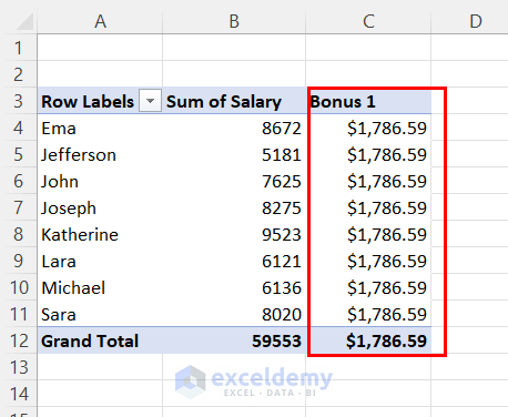
The Bonus 1 column with the bonuses of the employees will be automatically added to the PivotTable.

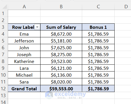
After adding the Currency symbol to the salaries and border to this table will have the final look like this figure.

Method 3 – Generating Explicit Calculated Field in Pivot Table Data Model

Use the Calculated Field directly to generate an explicit calculated field with a formula to determine the employees bonus amounts.

Steps:

• Follow Step-01 of Example-1 to open up the following sheet.

• Drag down Employee to the Rows area and Salary to the Values.

The following PivotTable will appear on the left side.

• After selecting any cell of your PivotTable, go to the PivotTable Analyze tab >> Calculations group >> Fields, Items & Sets dropdown >> Calculated Field

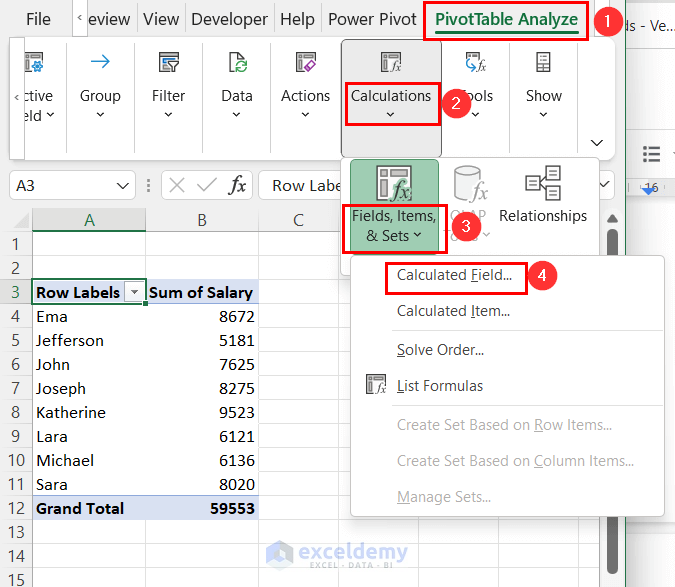
The Insert Calculated Field dialog box will pop up.

• Set the Name as Bonus 2.
• In the Formula box, after the equal sign (=) you will insert our desired field.

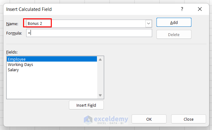
• Click on the Salary field and press the Insert Field.

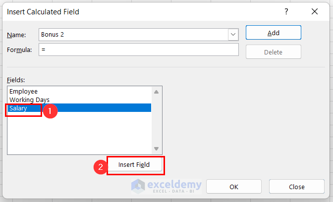
Salary will appear in the Formula box.

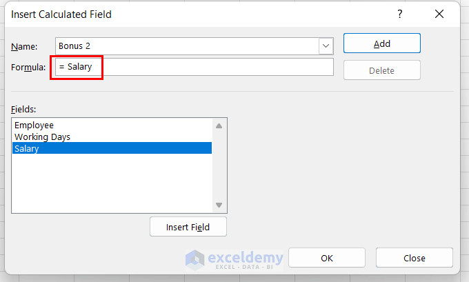
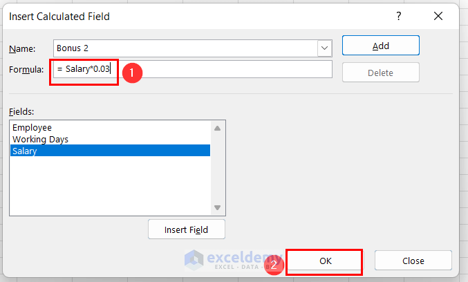
• Complete the formula like the following

• Press OK.

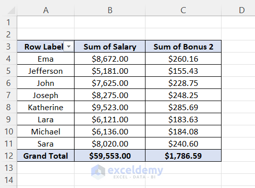
A new column with bonus values will be added to the Pivot Table.

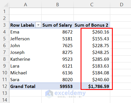
After adding the Currency symbol to the salaries and border to this table will have the final look like this figure.

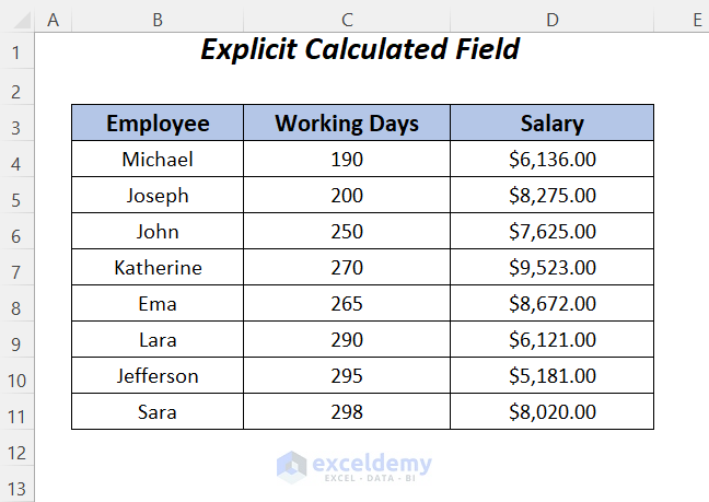
Method 4 –Using Explicit Calculated Field for a Complex Formula in Pivot Table Data Model

Steps:

• Follow Step-01 of Example-1 to open up the following sheet.

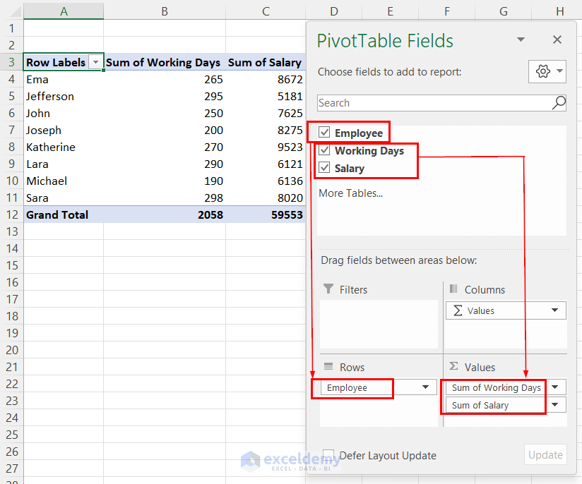
• Drag down Employee to the Rows area and Working Days, and Salary to the Values.

The following PivotTable will appear on the left side.

• After selecting any cell of your PivotTable, go to the PivotTable Analyze tab >> Calculations group >> Fields, Items & Sets dropdown >> Calculated Field.

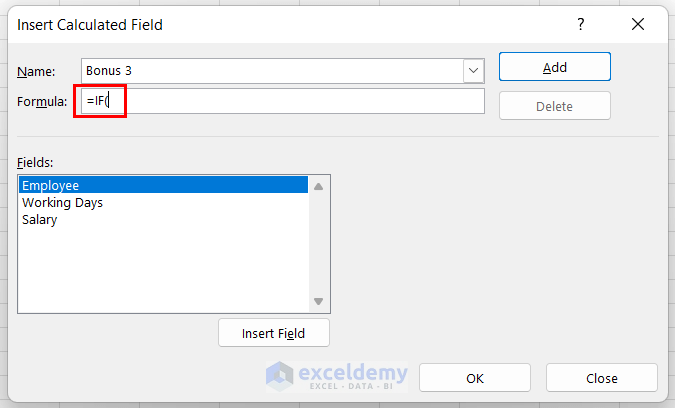
The Insert Calculated Field dialog box will pop up.

• Set the Name as Bonus 3.
• In the Formula box after the equal sign (=)you will insert our desired field here.

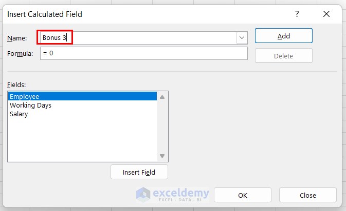
• Write down IF( to start the formula.

• Click on the Working Days field and press the Insert Field

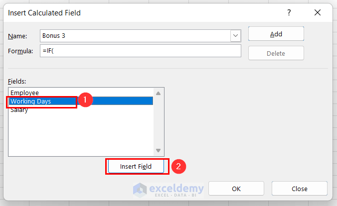
Insert the required fields into the formula.

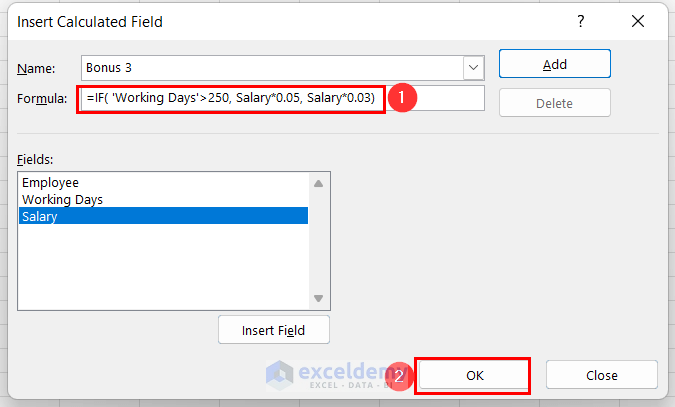
• Apply the following formula.

• Press OK.

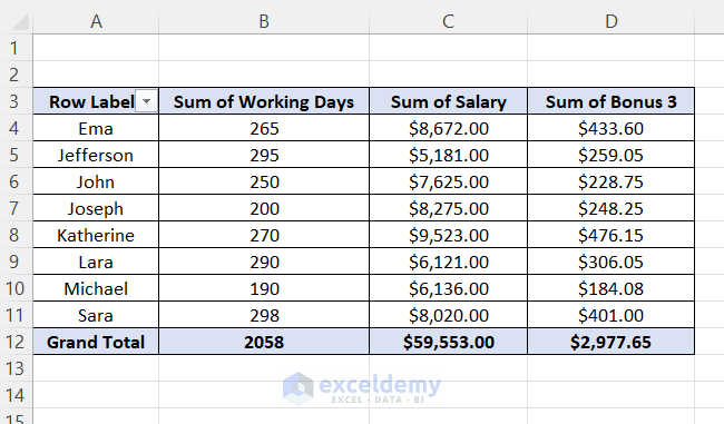
You will have a new column with calculated bonuses.

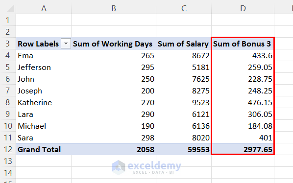
After adding the Currency symbol to the salaries, bonuses, and border to this table we will have the final look like this figure.

How to Remove Calculated Field in Pivot Table Data Model

Steps:

• Select any cell on the created column by entering the calculated field and then right-click on it.

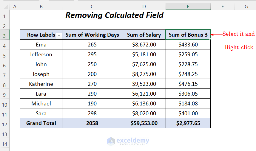
• Choose the Remove “Sum of Bonus 3”

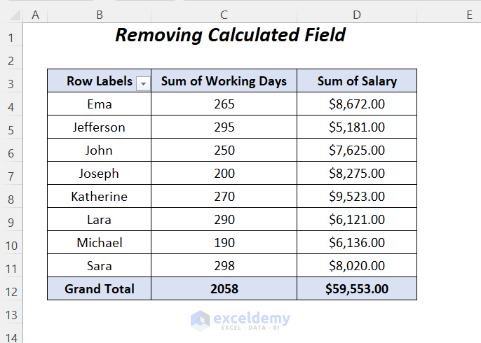
You removed the calculated field.

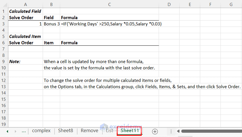
How to Get a List of Formulas for Calculated Field in Pivot Table Data Model

Steps:

• After selecting any cell of your PivotTable, go to the PivotTable Analyze tab >> Calculations group >> Fields, Items & Sets dropdown >> List Formulas

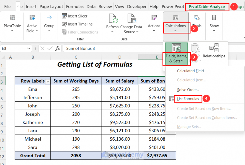
You will be taken to a new sheet for a detailed formula list.

Download Workbook

<< Go Back to Pivot Table Calculations | Pivot Table in Excel | Learn Excel