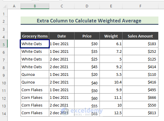
We have a dataset containing different grocery items and their sale details. We will calculate the weighted average price for each item in a Pivot Table.
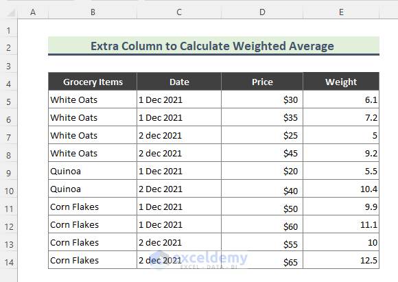
Step 1 – Adding a Helper Column
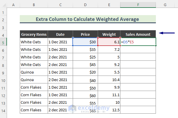
- Add a column Sales Amount in the above table.
- Use the following formula in the first cell of this new column.
=D5*E5- Hit Enter.
- Use the Fill Handle (+) tool to copy the formula to the rest of the column.
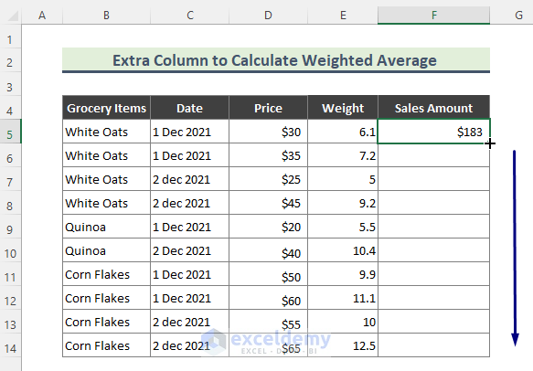
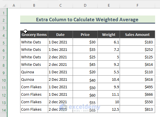
- You will get the following result.
Step 2 – Creating the Excel Pivot Table
- Click on any cell of the dataset (B4:F14).
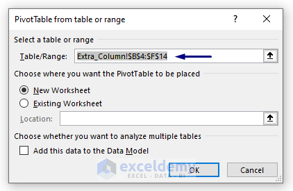
- Go to Insert and choose Pivot Table, then select From Table/Range.

- The PivotTable from table or range window will pop up. If your Table/Range field is correct, press OK.
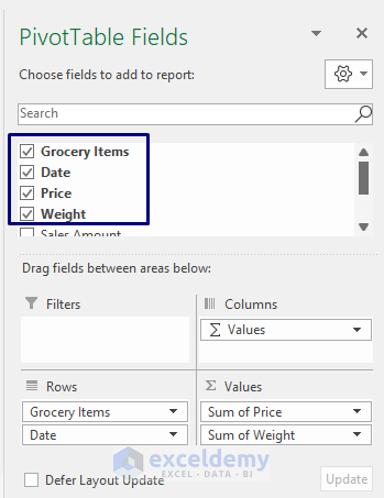
- The Pivot Table is created in a new sheet. Choose the PivotTable Fields as in the screenshot.
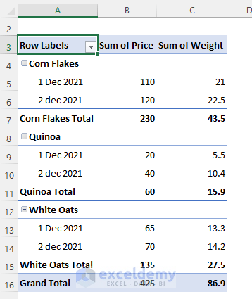
- You will get the following Pivot Table.
Step 3 – Analyzing the Weighted Average in an Excel Pivot Table
- Select the Pivot Table.
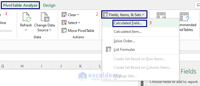
- Go to Pivot Table Analyze.
- Choose Field, Items, & Sets and select Calculated Field.
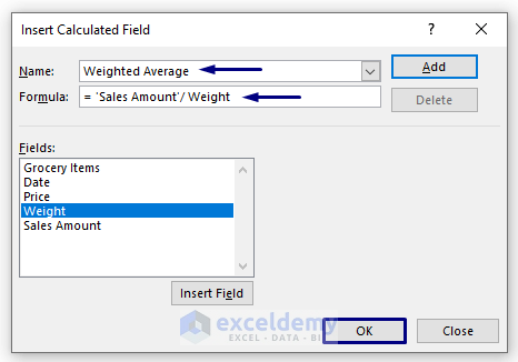
- The Insert Calculated Field window will show up.
- Type Weighted Average in the Name field.
- We have divided the helper column by weight (Sales Amount/Weight) to get the weighted average.
- Click on OK.
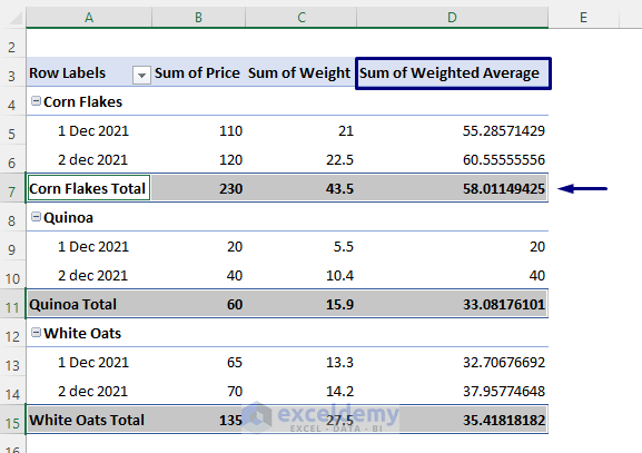
- We got the weighted average price for each of the grocery items in the subtotal rows of our Pivot Table.
Read More: Pivot Table Calculated Field for Average in Excel
Download the Practice Workbook
Related Articles
- Calculated Field Sum Divided by Count in Pivot Table
- How to Get a Count in Excel Pivot Table Calculated Field
- How to Apply Excel COUNTIF with Pivot Table Calculated Field
- How to Calculate Variance Using Pivot Table in Excel
<< Go Back to Pivot Table Calculations | Pivot Table in Excel | Learn Excel
Get FREE Advanced Excel Exercises with Solutions!
