How to Calculate the Variance Using a Pivot Table in Excel – Easy Steps

This is the dataset.

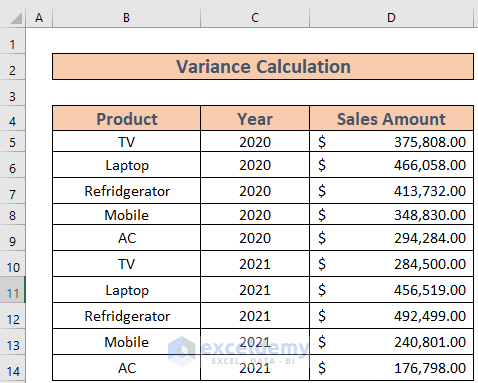
To calculate the variance of sales between 2020 and 2021:

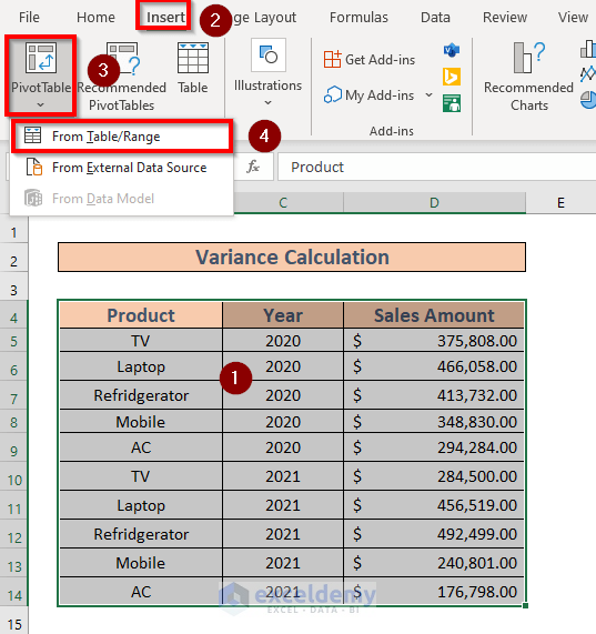
Step 1 – Create a Pivot Table from a Data Range

• Select B4:D14.
• Go to the Insert tab >> Pivot Table >> From Table/Range.

• In the new window, select New Worksheet to create a pivot table. Click OK.

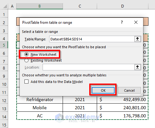
Excel will create a pivot table.

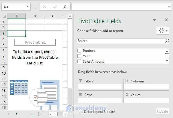
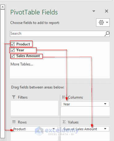
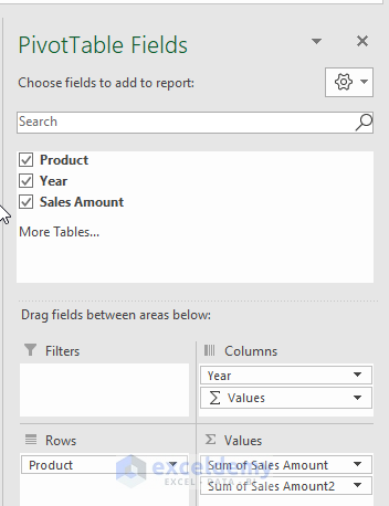
Step 2 – Drag the Fields

• In PivotTable Fields, enter Product in Rows, Year in Columns, and Sales Amount in Values

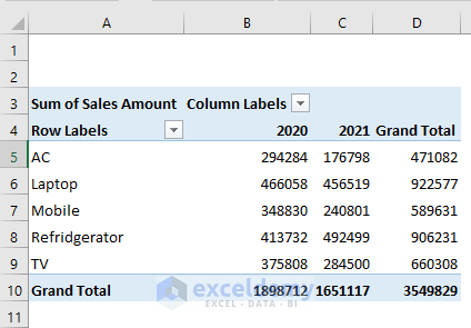
The table will be created.

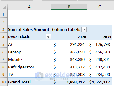
Step 3: Remove the Grand Total for Rows

• Go to Design >> select Layout >> select Grand Total >> choose On For Columns Only.

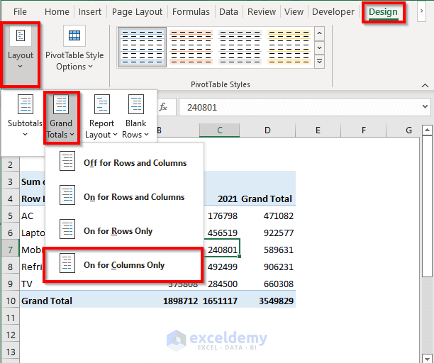
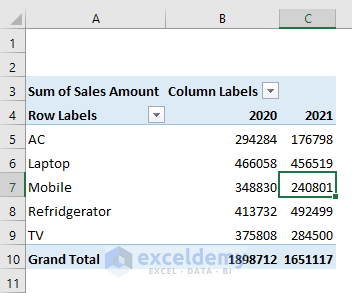
Excel will remove the Grand Total for Rows.

Step 4 – Change Cell Format to Accounting

• Select B5:D10.
• Go to the Home tab >> select the drop-down >> select More Number Formats.

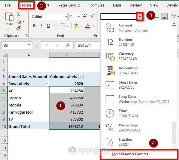
• In the Format Cells box, select Accounting >> set Decimal Places as 0 >> Click OK.

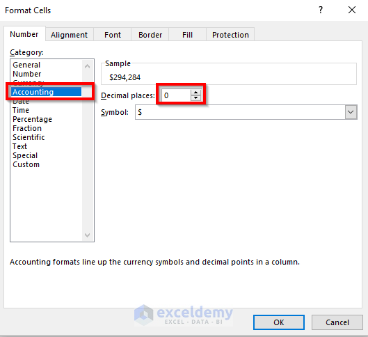
Excel will change the format of the sales amounts.

Step 5 – Calculate the Variance as a Change in Percentage

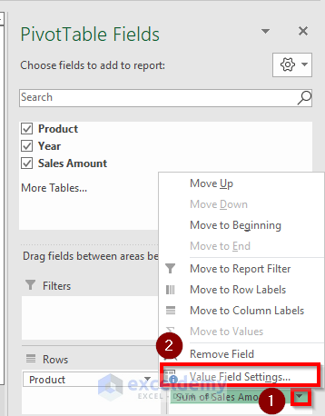
• Enter the Sales Amount in Values field.

• Select the drop-down shown below >> select Value Field Settings.

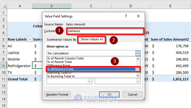
• In the Value Field Settings window, select Custom Name Variance >> select Show Values as >> choose % Difference From.

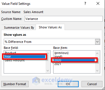
• Select the Base field as Year and the Base item as 2020.
• Click OK.

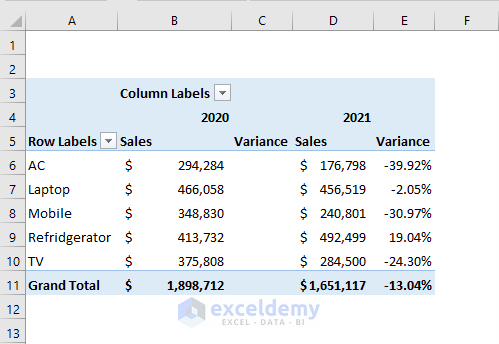
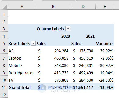
Excel will calculate the variance.

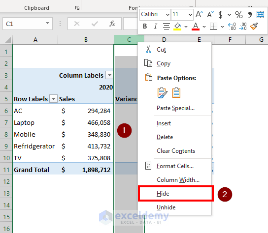
• Select column C.
• Choose Hide.

This is the output.

Things to Remember

• This variance is different from statistical variance.

Download Practice Workbook

Download the workbook and practice.

Related Articles

• Pivot Table Calculated Field for Average in Excel
• Calculated Field Sum Divided by Count in Pivot Table
• How to Get a Count in Excel Pivot Table Calculated Field
• How to Apply Excel COUNTIF with Pivot Table Calculated Field
• How to Calculate Weighted Average in Excel Pivot Table

<< Go Back to Pivot Table Calculations | Pivot Table in Excel | Learn Excel