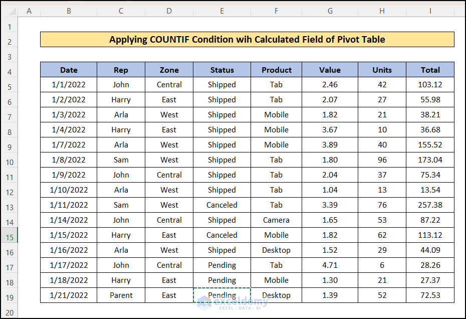
The dataset showcases sales information.
Calculate the number of days with total sales greater than 100 units:
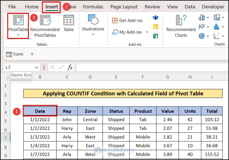
Step 1 – Create a Pivot Table
- Click any cell in the dataset and go to the Insert tab.
- Select PivotTable.
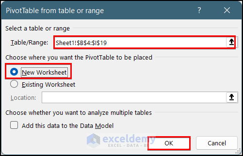
- Select New Worksheet or Existing Worksheet to insert the pivot table.
- Click OK.
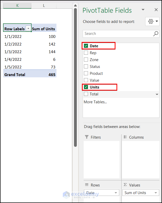
- A blank pivot table will be created.
- In the PivotTable Fields window, check Date and Units.
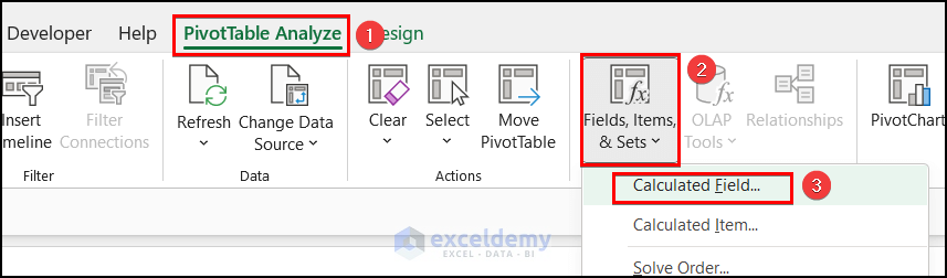
- Click the pivot table and go to PivotTable Analyze.
- Click Fields, Items & Sets and select Calculated Field.
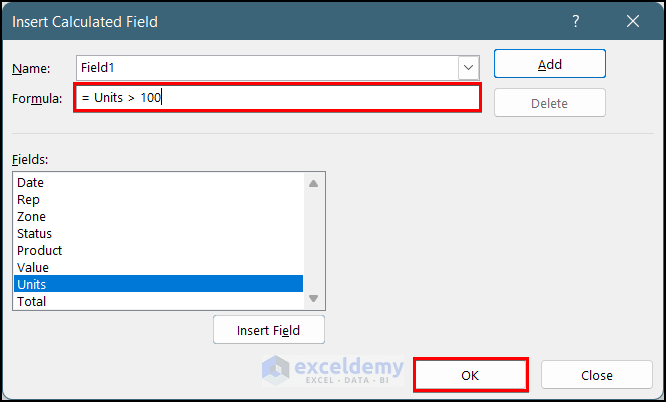
Step 2 – Insert a Calculated Field in the Pivot Table
- In the “Insert Calculated Field” window, enter the following formula.
= Units > 100Note:
You can insert the fields by selecting them from the lists and clicking Insert Variable.
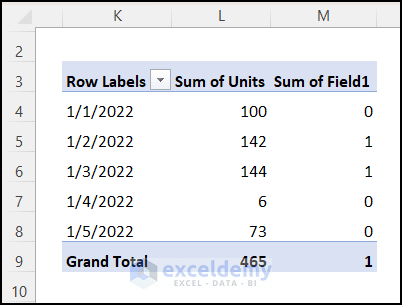
- A new column is created in the pivot table.
- In this column, 1 refers to sales greater than 100 units on that day.
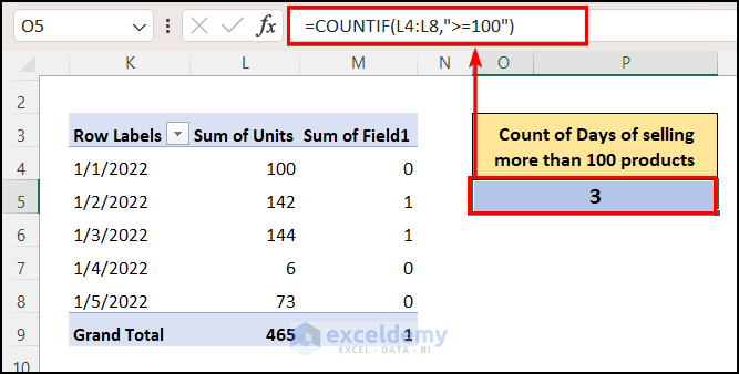
Final Step: Use the COUNTIF Function with a Calculated Field Column
- Enter the following formula to calculate the count of days with sales greater than 100 units per day.
=COUNTIF(L4:L8,">=100")
Read More: How to Get a Count in Excel Pivot Table Calculated Field
How to Use an Excel If Statement in a Pivot Table Calculated Field
In the calculated field of the pivot table, it’s not possible to use Excel functions like IF or COUNTIF. To count or sum use the Formula box without Excel functions.
Download Practice Workbook
Download the practice workbook here.
Related Articles
- Pivot Table Calculated Field for Average in Excel
- Calculated Field Sum Divided by Count in Pivot Table
- How to Calculate Weighted Average in Excel Pivot Table
- How to Calculate Variance Using Pivot Table in Excel
<< Go Back to Pivot Table Calculations | Pivot Table in Excel | Learn Excel
Get FREE Advanced Excel Exercises with Solutions!
