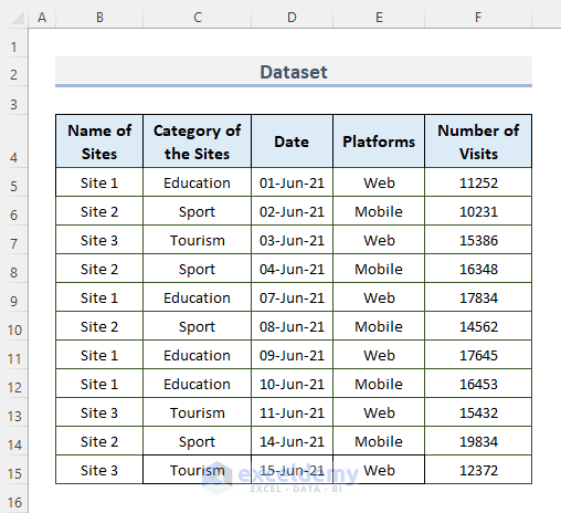
This is the sample dataset.
Method 1 – Combine Excel MIN & IF Functions to Get the Lowest Value
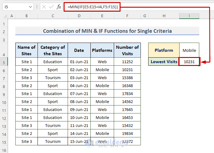
1.1. Single Criteria
To get the lowest visits of the platform Mobile in F5:F15:
STEPS:
- Select a cell and enter the formula:
=MIN(IF(E5:E15=I4,F5:F15))
- Press Enter.
Formula Breakdown
E5:E15 is the platforms, I4 is Mobile, and F5:F15 is the number of visits.
Read More: How to Use Combined MIN and IF Function in Excel
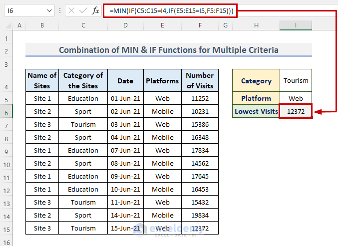
1.2. Multiple Criteria
STEPS:
- Select a cell and enter the formula:
=MIN(IF(C5:C15=I4,IF(E5:E15=I5,F5:F15)))
- Press Enter.
Formula Breakdown
C5:C15 is the category of the sites, I4 is a category : Tourism, E5:E15 is platforms, I6 is a mode of platforms: Web, and F5:F15 is the number of visits.
Read more: How to Find Minimum Value in Excel
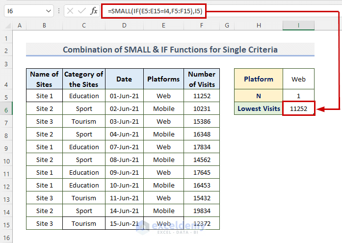
Method 2 – Merge the SMALL & IF Functions to Find the Minimum Value
2.1. Single Criteria
STEPS:
- Select a cell and enter the formula:
=SMALL(IF(E5:E15=I4,F5:F15),I5)
- Press Enter.
Formula Breakdown
E5:E15 is platforms, I4 is a mode of platforms: Web, F5:F15 is the number of visits, and N is 1 for the lowest value.
2.2. Multiple Criteria with OR Logic
STEPS:
- Select a cell and enter the formula:
=SMALL(IF((E5:E15=I4) + (E5:E15=I5), F5:F15), I6)
- Press Enter.
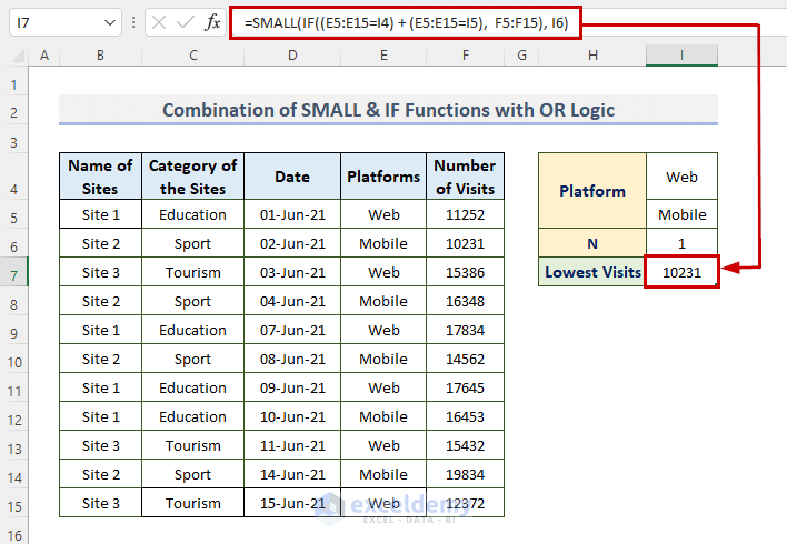
Formula Breakdown
E5:E15 is platforms, I4 is a mode of platforms: Web, I5 is another mode of platform: Mobile, F5:F15 is the number of visits, and I6 is 1, the value of N.
2.3. Multiple Criteria with AND Logic
STEPS:
- Select a cell and enter the formula:
=SMALL(IF((B5:B15=I4) * (E5:E15=I5), F5:F15), I6)
- Press Enter.
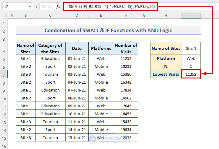
Formula Breakdown
B5:B15 is the name of sites, I4 is site 1, E5:E15 is platforms, I5 is Web, F5:F15 is thenumber of visits, and I6 is 1, the value of N.
Method 3 – Integrate the INDEX, MATCH & MIN Functions in Excel
STEPS:
- Select a cell and enter the formula:
=INDEX(B5:F15, MATCH(MIN(F5:F15), F5:F15, 0 ), 5 )
- Press Enter.
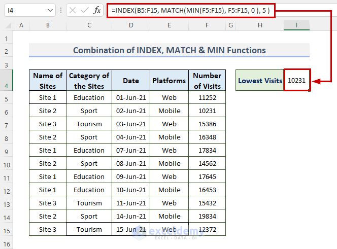
Formula Breakdown
B5:B15 is the name of sites, F5:F15 is the number of visits, 5 is the column position of the number of visits.
Method 4 – Combining the INDEX, MATCH & SMALL Functions to find the Lowest Value with Criteria
STEPS:
- Select a cell and enter the formula:
=INDEX($C$5:$C$15, MATCH(SMALL($F$5:$F$15, I4), $F$5:$F$15, 0))
- Press Enter.
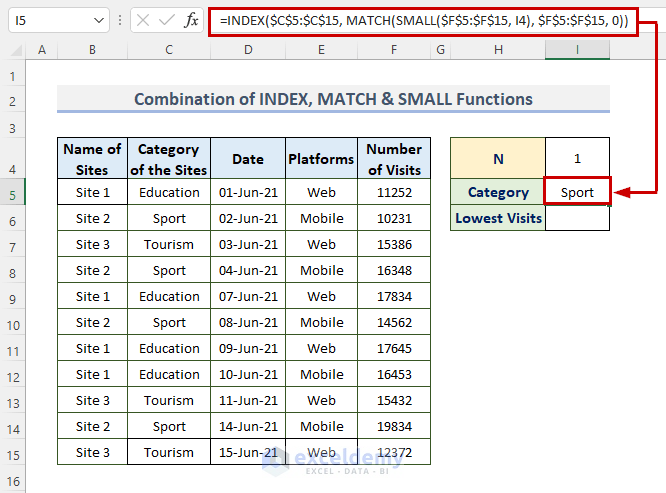
To get the lowest value use the following formula.
=INDEX($F$5:$F$15, MATCH(SMALL($F$5:$F$15, I4), $F$5:$F$15, 0))
- Press Enter.
Formula Breakdown
The formula searches for the smallest value and matches it with the category, returning the result.
Read More: How to Find Lowest 3 Values in Excel
Method 5 – Using the Excel AGGREGATE Function to find the Lowest Value with Criteria
STEPS:
- Select a cell and enter the formula:
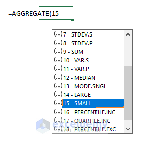
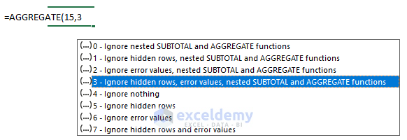
=AGGREGATE(15,3,1/((C5:C15=I4)*(E5:E15=I5))*F5:F15,1)
- Press Enter.

Formula Breakdown
15 is used to find the Smallest option among 19 options, 3 is used to ignore hidden rows, error values, etc., C5:C15 is the category of the sites, I4 is Sport, E5:E15 is the mode of platforms, I5 is Mobile, F5:F15 is the number of visits, 1 is the value of N.
15 was selected to get the smallest value.
3 ignores hidden rows, error values, and nested SUBTOTAL, and AGGREGATE functions.
Method 6 – Using the MINIFS Function to Get the Lowest Value in Excel
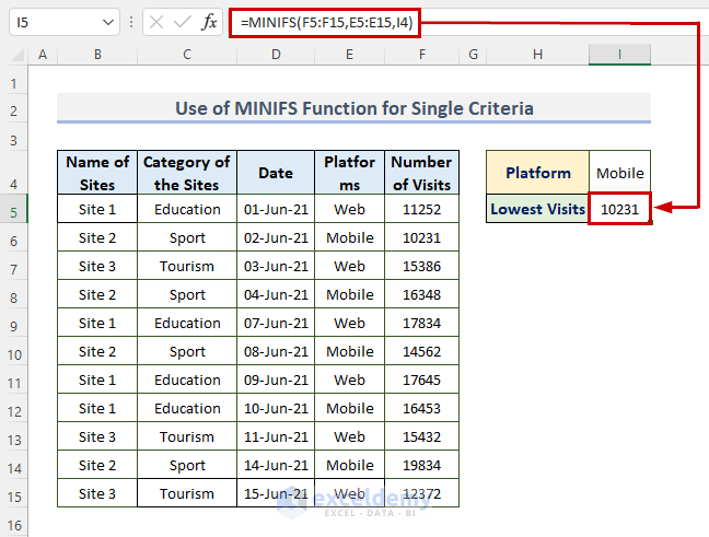
6.1. Single Criteria
STEPS:
- Select a cell and enter the formula:
=MINIFS(F5:F15,E5:E15,I4)
- Press Enter.
Formula Breakdown
F5:F15 is the number of visits, E5:E15 is the mode of platforms, and I4 is Mobile.
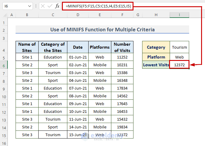
6.2. Multiple Criteria
STEPS:
- Select a cell and enter the formula:
=MINIFS(F5:F15,C5:C15,I4,E5:E15,I5)
- Press Enter.
Formula Breakdown
F5:F15 is the number of visits, C5:C15 is the category, I4 is Tourism, E5:E15 is the mode of platforms, and I6 is Web.
Read More: How to Find Minimum Value Based on Multiple Criteria in Excel
Method 7 – Joining the VLOOKUP & MIN Functions to Find the Lowest Value
STEPS:
- Select a cell and enter the formula:
=VLOOKUP(MIN($C$5:$C$15),$C$5:$D$15, 2, 0)
- Press Enter.
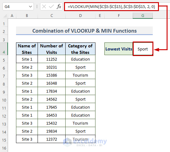
Formula Breakdown
MIN locates the lowest value in a range. Use a range or a row to apply the VLOOKUP search.
Read More: How to Find Minimum Value with VLOOKUP in Excel
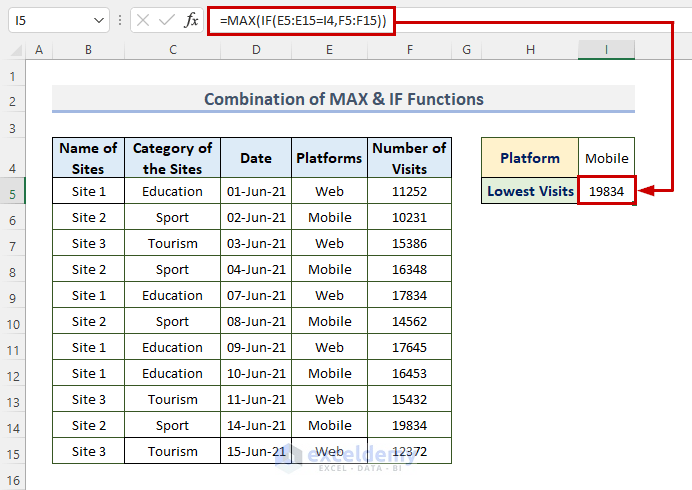
How to Find the Highest Value with Criteria in Excel
STEPS:
- Select a cell and enter the formula:
=MAX(IF(E5:E15=I4,F5:F15))
- Press Enter.
Download Practice Workbook
Related Articles
- How to Use MIN Function to Exclude Zero in Excel
- Excel MIN Function Returns 0
- How to Find Minimum Value That Is Greater Than 0 in Excel
- Difference Between MAX and MIN Function in Excel
<< Go Back to Excel MIN Function | Excel Functions | Learn Excel
Get FREE Advanced Excel Exercises with Solutions!
