Method 1 – INDIRECT Function with Sheet Name to Refer Another Worksheet
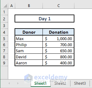
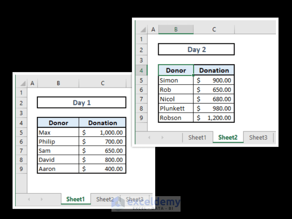
In the example image below, Sheet1 contains the names of donors and the donation.
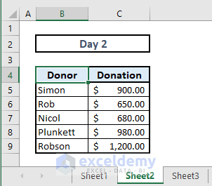
Sheet2 represents another chart for Day 2.
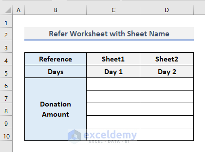
In Sheet3, the data from the previous two sheets will be extracted.
In Cell C6, insert the formula below:
=INDIRECT(C4&"!C5:C9")Press Enter to get the donation amounts in an array from Sheet1.
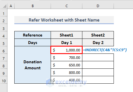
In this formula, the INDIRECT function uses the cell reference C4 as an input value which contains the sheet name of the first sheet. With the use of Ampersand (&), the other necessary symbols have been used to refer to a particular range of cells from another worksheet.
To get an array of donation amounts in Column D, we have to use the following formula in Cell D6:
=INDIRECT(D4&"!C5:C9")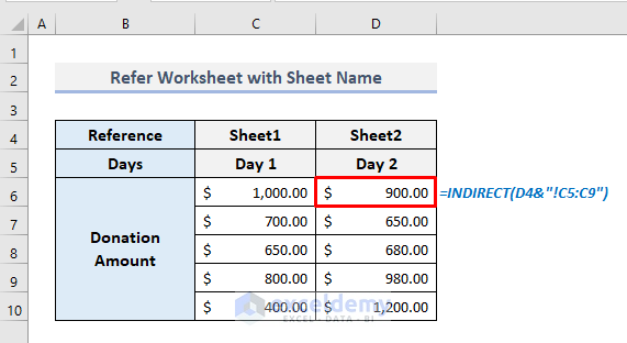
Read More: How to Use Excel INDIRECT Range
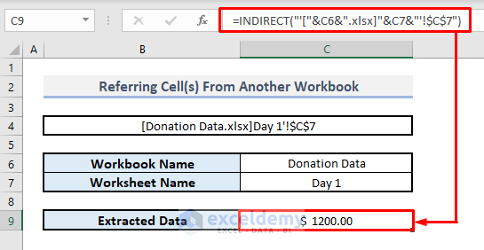
Method 2 – INDIRECT Function to Refer Sheet Name from Another Workbook in Excel
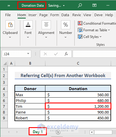
Step 1:
➤ Open a new workbook.
➤ In Cell B4, type ‘=’ and click on Cell C7 of the Donation Data workbook.
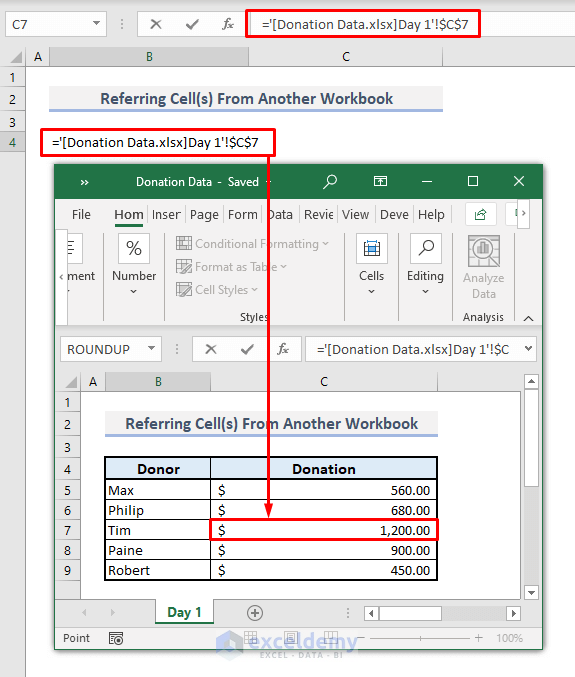
Step 2:
➤ Press Enter and the value of $1200 will be shown.
➤ Keep this Cell B4 in text format. Remove the Equal(=) symbol from the cell.
.➤ In Cells C6 and C7, type the names of the Excel workbook and the spreadsheet respectively from where the data will be extracted.
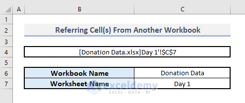
Step 3:
➤ In Cell C9, enter:
=INDIRECT("'["&C6&".xlsx]"&C7&"'!$C$7")➤ Press Enter.
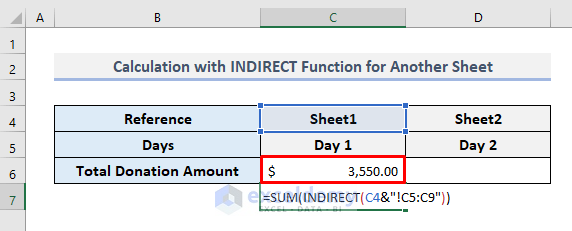
Method 3 – Numeric Calculation with INDIRECT Function While Referring to a Sheet Name
To calculate the total donation amount for Day 1 by using the SUM function before the INDIRECT function, insert the formula below in
Cell C6:
=SUM(INDIRECT(C4&”!C5:C9″))
Press Enter, the formula will return the expected total.
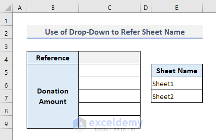
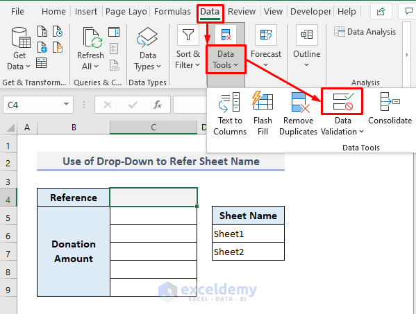
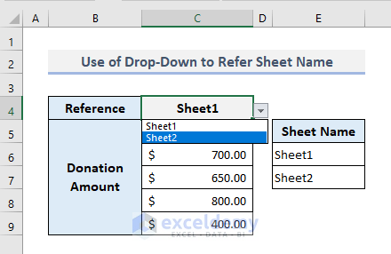
Method 4 – Use of Drop Down to Input Sheet Name in the INDIRECT Function in Excel
Step 1:
➤Select Cell C4.
➤ Under Data, choose the Data Validation command from the drop-down.
A dialogue box will open up.
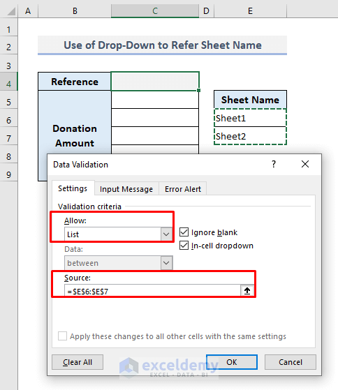
Step 2:
➤ In the Allow box, choose List from the options.
➤ Enable editing in the Source box and select the range of cells (E6:E7) containing the sheet names.
➤ Press OK.
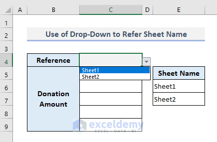
Our required drop-down list in Cell C4 is now ready to show the assigned values. Assuming that we have selected the option Sheet1 from the drop-down.
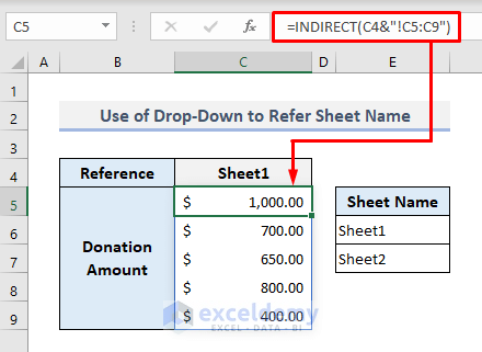
Step 3:
➤ In the output Cell C5, insert the following formula:
=INDIRECT(C4&"!C5:C9")➤ Press Enter.
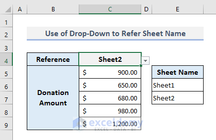
Step 4:
➤ Select another option (Sheet2) from the drop-down list now.
The output in the range of cells (C5:C9) will be updated.
Download Practice Workbook
Related Articles
- Create Drop-Down List Using INDIRECT Function in Excel
- How to Use Indirect Address in Excel
- INDIRECT Function to Get Values from Different Sheet in Excel
- How to Convert Text to Formula Using the INDIRECT Function in Excel
<< Go Back to Excel INDIRECT Function | Excel Functions | Learn Excel
Get FREE Advanced Excel Exercises with Solutions!
