Excel VBA to Highlight Specific Text in a Cell (6 Ways)

Download Practice Workbook

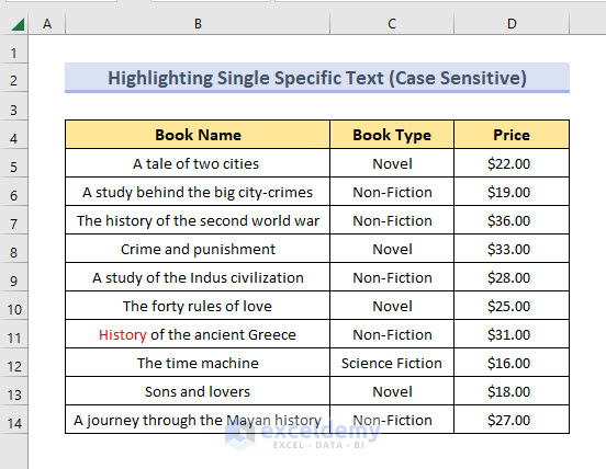
We will use VBA codes to highlight specific text in the sample data set below.

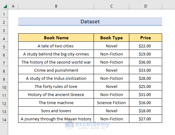
Method 1 – VBA Code to Highlight a Single Specific Text in a Range of Cells in Excel (Case-Insensitive Match)

• Develop a Macro to highlight a single specific text from a range of cells in the data set, with a case-insensitive match.
• We will highlight the text “history” from the names of the books.
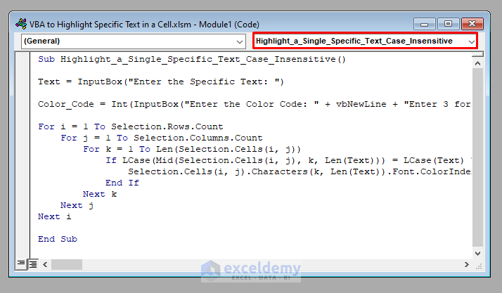
• Enter the following VBA code.

⧭ VBA Code:

Sub Highlight_a_Single_Specific_Text_Case_Insensitive()

Text = InputBox("Enter the Specific Text: ")

Color_Code = Int(InputBox("Enter the Color Code: " + vbNewLine + "Enter 3 for Color Red." + vbNewLine + "Enter 5 for Color Blue." + vbNewLine + "Enter 6 for Color Yellow." + vbNewLine + "Enter 10 for Color Green."))

For i = 1 To Selection.Rows.Count
    For j = 1 To Selection.Columns.Count
        For k = 1 To Len(Selection.Cells(i, j))
            If LCase(Mid(Selection.Cells(i, j), k, Len(Text))) = LCase(Text) Then
                Selection.Cells(i, j).Characters(k, Len(Text)).Font.ColorIndex = Color_Code
            End If
        Next k
    Next j
Next i

End Sub

⧭ Step-by-Step Procedure to Run the Code:

Step 1: Opening the VBA Window

• Press ALT + F11 to open the VBA window.

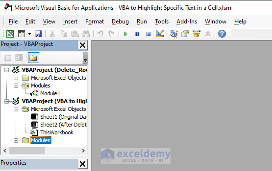
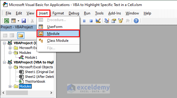
Step 2: Inserting a New Module

• In the VBA toolbar, go to the Insert > Module.
• Click on Insert. A new module called “Module 1” will be inserted.

Step 3: Entering the VBA Code

• Enter the following VBA code into the new module.

Step 4: Saving Macro-Enabled Workbook

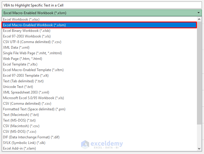
• Save the workbook as Excel Macro-Enabled Workbook.

Step 5: Running the VBA Code

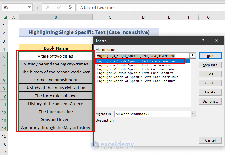
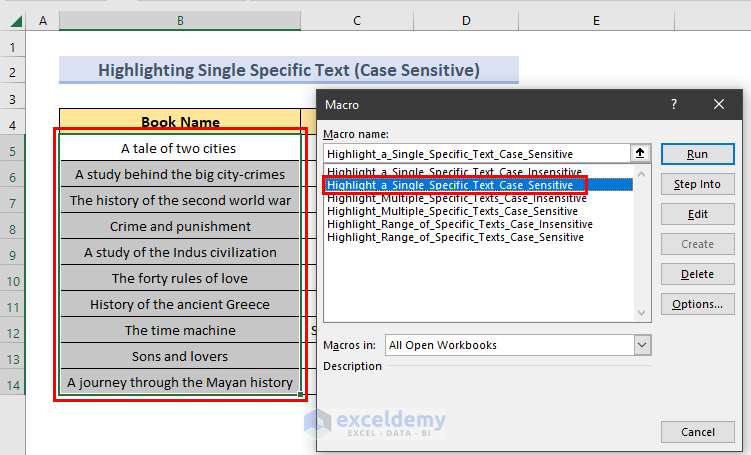
• Back on the worksheet, select the range to highlight the specific text. We have selected the column Book Name.
• Press ALT+F8. A dialogue box named Macro will open.
• Select Highlight_a_Single_Specific_Text_Case_Insensitive and click on Run.

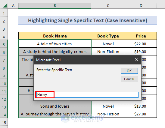
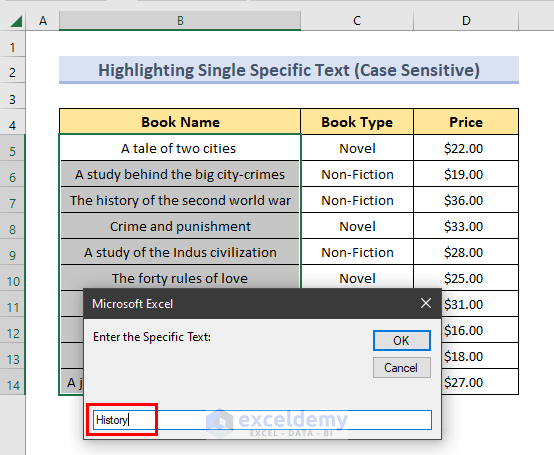
Step 6: Entering the Inputs

• You will get two Input boxes. The first box will ask you to enter the specific text to highlight. We have entered “History”.

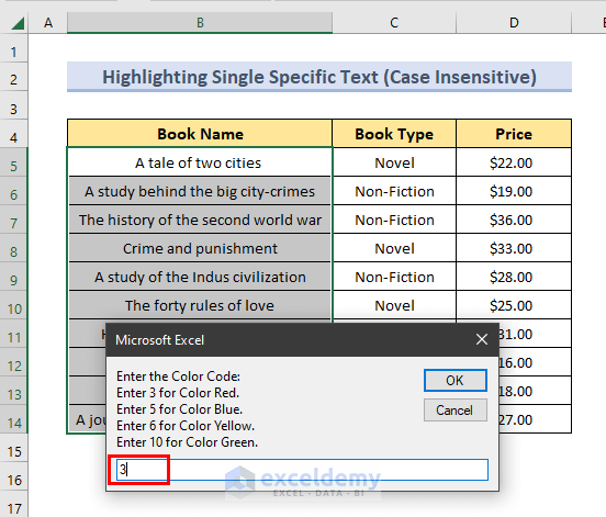
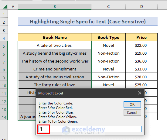
• The 2nd box will ask you to enter the color to highlight the text.
• Enter 3 for a red, 5 for a blue, 6 for a yellow and 10 for green or enter any other color code according to the table provided by Microsoft.
• We have entered 3 (Red).

Step 7: The Final Output

• Click OK. You’ll get all the instances of the text “History” highlighted in red in your selected range.

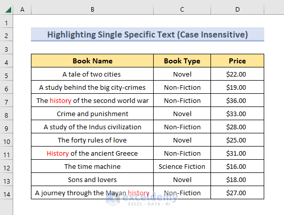The code is case-insensitive. So, it will highlight all occurrences of the search term ‘history,’ including ‘History,’ ‘HISTORY,’ etc.

Read More: How to Highlight Selected Text in Excel (8 Ways)

Method 2 – VBA Code to Highlight a Single Specific Text in a Range of Cells in Excel (Case-Sensitive Match)

• Create a new module and enter the following VBA code as shown in Method 1.

⧭ VBA Code:

Sub Highlight_a_Single_Specific_Text_Case_Sensitive()

Text = InputBox("Enter the Specific Text: ")

Color_Code = Int(InputBox("Enter the Color Code: " + vbNewLine + "Enter 3 for Color Red." + vbNewLine + "Enter 5 for Color Blue." + vbNewLine + "Enter 6 for Color Yellow." + vbNewLine + "Enter 10 for Color Green."))

For i = 1 To Selection.Rows.Count
    For j = 1 To Selection.Columns.Count
        For k = 1 To Len(Selection.Cells(i, j))
            If Mid(Selection.Cells(i, j), k, Len(Text)) = Text Then
                Selection.Cells(i, j).Characters(k, Len(Text)).Font.ColorIndex = Color_Code
            End If
        Next k
    Next j
Next i

End Sub

⧭ Steps to Run the Code:

• Run the code as shown in Method 1.
• Create a new module and insert the code.

• Save the workbook as Excel Macro-Enabled Workbook. Come back to your worksheet, select the range of cells and run the Macro named Highlight_a_Single_Specific_Text_Case_Sensitive.

• You will get two input boxes. Enter the text (“History”) in the 1st box.

• Enter the color code (3 in this example) in the 2nd box.

• Click OK. You’ll find the instances of the text “history” highlighted red in your worksheet.

This is a case-sensitive code. So only the text “history” will be highlighted, not “History” or anything else.

Read More: Highlight Cells That Contain Text from a List in Excel (7 Easy Ways)

Method 3 – VBA Code to Highlight Multiple Specific Texts in a Range of Cells in Excel (Case-Insensitive Match)

• Create a new module and enter the following VBA code.

⧭ VBA Code:

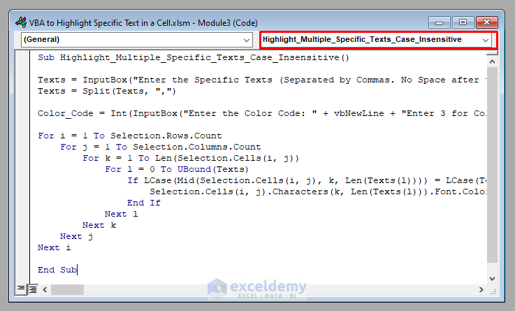
Sub Highlight_Multiple_Specific_Texts_Case_Insensitive()

Texts = InputBox("Enter the Specific Texts (Separated by Commas. No Space after the Commas): ")

Texts = Split(Texts, ",")

Color_Code = Int(InputBox("Enter the Color Code: " + vbNewLine + "Enter 3 for Color Red." + vbNewLine + "Enter 5 for Color Blue." + vbNewLine + "Enter 6 for Color Yellow." + vbNewLine + "Enter 10 for Color Green."))

For i = 1 To Selection.Rows.Count
    For j = 1 To Selection.Columns.Count
        For k = 1 To Len(Selection.Cells(i, j))
            For l = 0 To UBound(Texts)
                If LCase(Mid(Selection.Cells(i, j), k, Len(Texts(l)))) = LCase(Texts(l)) Then
                    Selection.Cells(i, j).Characters(k, Len(Texts(l))).Font.ColorIndex = Color_Code
                End If
            Next l
        Next k
    Next j
Next i

End Sub

⧭ Steps to Run the Code:

• Run the code as shown in Method 1.
• Create a new module and insert the code.

• Save the workbook as Excel Macro-Enabled Workbook.
• Back on your worksheet, select the range of cells and run the Macro called Highlight_Multiple_Specific_Texts_Case_Insensitive.

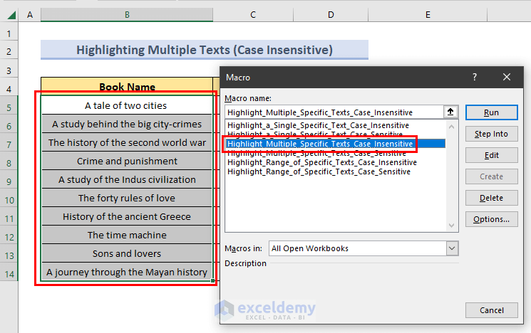
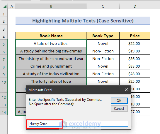
• You will get two input boxes. In the 1st box, enter the specific texts separated by commas (No space after the commas).
• We have entered history,crime.

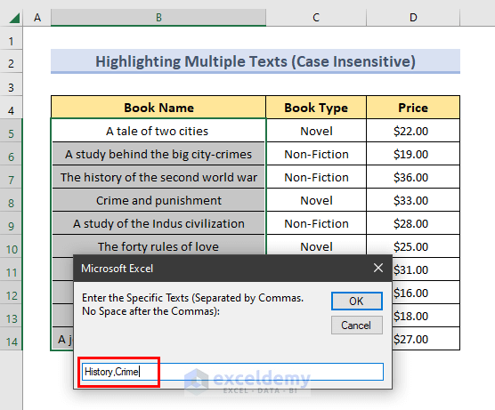
• Enter the color code (10 in this example) in the 2nd box.

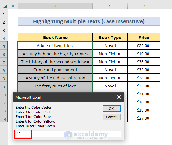
• Click OK. You’ll find the instances of the texts “history” and “crime” highlighted green in your worksheet.

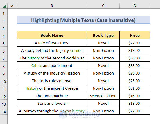
This is a case-insensitive code. So, “history”, “History”, “crime”, “Crime” have been highlighted.

Similar Readings

• Compare Two Excel Sheets and Highlight Differences (7 Ways)
• How to Highlight a Row in Excel (2 Effective Ways)
• Highlight Cells Based on Text in Excel [2 Methods]

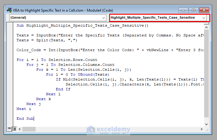
Method 4 – VBA Code to Highlight Multiple Specific Texts in a Range of Cells in Excel (Case-Sensitive Match)

• Create a new module and enter the following VBA code.

⧭ VBA Code: 

Sub Highlight_Multiple_Specific_Texts_Case_Sensitive()

Texts = InputBox("Enter the Specific Texts (Separated by Commas. No Space after the Commas): ")

Texts = Split(Texts, ",")

Color_Code = Int(InputBox("Enter the Color Code: " + vbNewLine + "Enter 3 for Color Red." + vbNewLine + "Enter 5 for Color Blue." + vbNewLine + "Enter 6 for Color Yellow." + vbNewLine + "Enter 10 for Color Green."))

For i = 1 To Selection.Rows.Count
    For j = 1 To Selection.Columns.Count
        For k = 1 To Len(Selection.Cells(i, j))
            For l = 0 To UBound(Texts)
                If Mid(Selection.Cells(i, j), k, Len(Texts(l))) = Texts(l) Then
                    Selection.Cells(i, j).Characters(k, Len(Texts(l))).Font.ColorIndex = Color_Code
                End If
            Next l
        Next k
    Next j
Next i

End Sub

⧭ Steps to Run the Code:

• Run the code as shown in Method 1.
• Create a new module and insert the code.

• Save the workbook as Excel Macro-Enabled Workbook, come back to your worksheet, select the range of cells and run the Macro called Highlight_Multiple_Specific_Texts_Case_Sensitive.

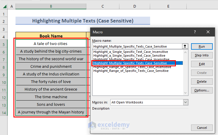
• You will get two input boxes. In the 1st box, enter the specific texts separated by commas (No space after the commas). We have entered history,crime.

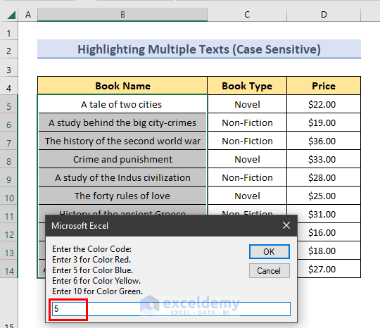
• Enter the color code (5 in this example) in the 2nd box.

• Click OK. You’ll find the instances of the texts “history” and “crime” highlighted blue in your worksheet.

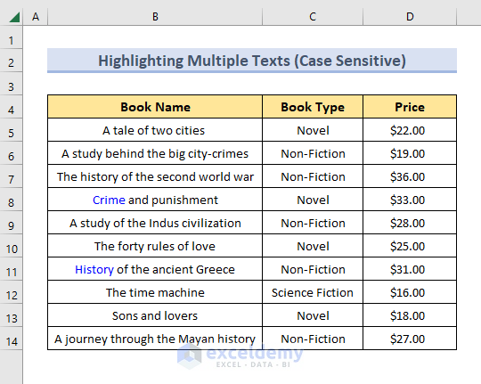
This is a case-sensitive code. So only “history”, “crime”, and “love” have been highlighted.

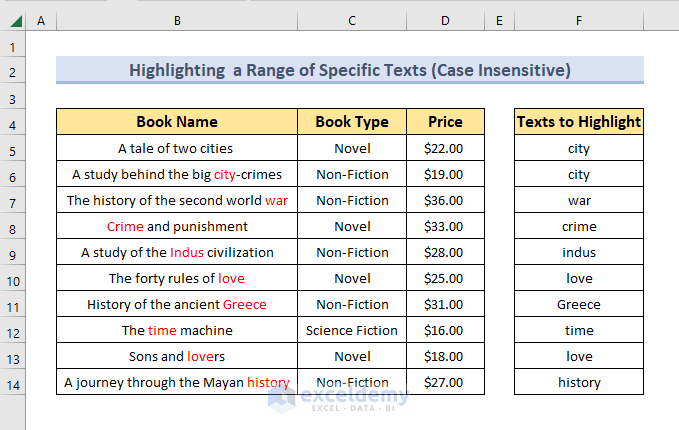
Method 5 – VBA Code to Highlight a Range of Specific Texts in a Range of Cells in Excel (Case-Insensitive Match)

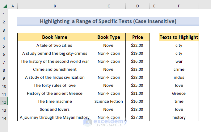
In the sample dataset, there is an extra column called Texts to Highlight. We’ll match each text value from this column with the corresponding text value of the Book Name column. Also, highlight the portion in the book name if the corresponding text value is found in the name.

• Create a new module and insert the following VBA code.

⧭ VBA Code:

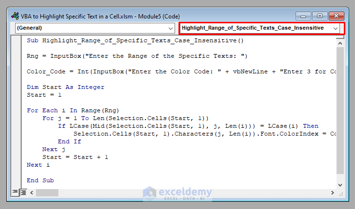
Sub Highlight_Range_of_Specific_Texts_Case_Insensitive()

Rng = InputBox("Enter the Range of the Specific Texts: ")

Color_Code = Int(InputBox("Enter the Color Code: " + vbNewLine + "Enter 3 for Color Red." + vbNewLine + "Enter 5 for Color Blue." + vbNewLine + "Enter 6 for Color Yellow." + vbNewLine + "Enter 10 for Color Green."))

Dim Start As Integer
Start = 1

For Each i In Range(Rng)
    For j = 1 To Len(Selection.Cells(Start, 1))
        If LCase(Mid(Selection.Cells(Start, 1), j, Len(i))) = LCase(i) Then
            Selection.Cells(Start, 1).Characters(j, Len(i)).Font.ColorIndex = Color_Code
        End If
    Next j
    Start = Start + 1
Next i

End Sub

⧭ Steps to Run the Code:

• Run the code as shown in Method 1.
• Create a new module and insert the code.

• Save the workbook as Excel Macro-Enabled Workbook, come back to your worksheet, select the range of cells and run the Macro called Highlight_Range_of_Specific_Texts_Case_Insensitive.

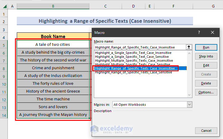
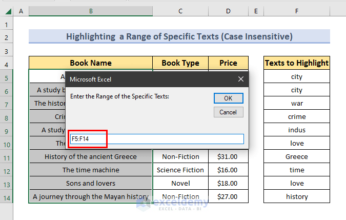
• Two input boxes will open. In the 1st box, enter the range of the specific texts to match. In this example, it’s F5:F14.

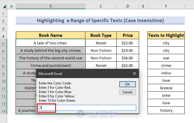
• Enter the color code (3 in this example) in the 2nd box.

• Click OK. You’ll find the instances highlighted in red where any portion of the book name matches the corresponding text value (With case-insensitive match).

Read More: Excel VBA to Highlight Cell Based on Value (5 Examples)

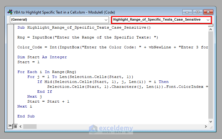
Method 6 – VBA Code to Highlight a Range of Specific Texts in a Range of Cells in Excel (Case-Sensitive Match)

Create a new module and insert the following VBA code.

⧭ VBA Code:

Sub Highlight_Range_of_Specific_Texts_Case_Sensitive()

Rng = InputBox("Enter the Range of the Specific Texts: ")

Color_Code = Int(InputBox("Enter the Color Code: " + vbNewLine + "Enter 3 for Color Red." + vbNewLine + "Enter 5 for Color Blue." + vbNewLine + "Enter 6 for Color Yellow." + vbNewLine + "Enter 10 for Color Green."))

Dim Start As Integer
Start = 1

For Each i In Range(Rng)
    For j = 1 To Len(Selection.Cells(Start, 1))
        If Mid(Selection.Cells(Start, 1), j, Len(i)) = i Then
            Selection.Cells(Start, 1).Characters(j, Len(i)).Font.ColorIndex = Color_Code
        End If
    Next j
    Start = Start + 1
Next i

End Sub

• Follow the steps shown in Method 1 and the output will be as shown in the image below.

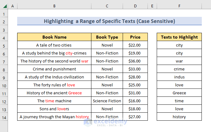
• Only the case-sensitive matches will be highlighted.

Related Readings

• How to Highlight Text in Text Box in Excel (3 Handy Ways)
• Excel Cell Color: Add, Edit, Use & Remove
• How to Highlight Partial Text in Excel Cell (9 Methods)
• VBA to Change Cell Color Based on Value in Excel (3 Easy Examples)
• How to Highlight a Cell in Excel (5 Methods)