Highlight Cells That Contain Text from a List in Excel (7 Easy Ways)

Method 1 – Use the COUNTIF Function to Highlight Cells That Have Text from a List

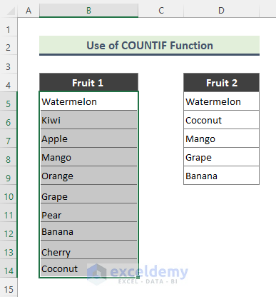
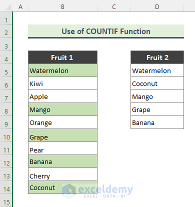
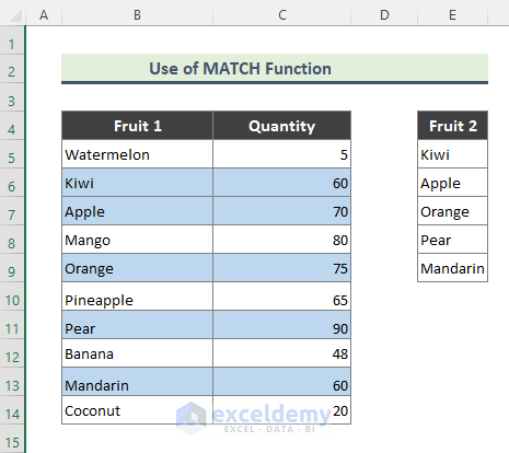
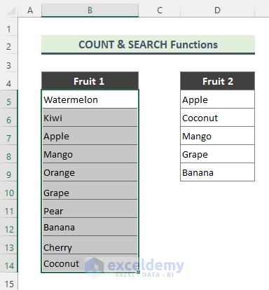
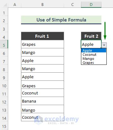
We have a list of Fruit 1 (B4:B14) containing several fruit names. In another list, Fruit 2 (D4:D9), we have some other fruit names. We will highlight the names from Fruit 2 in the list Fruit 1.

Steps:

• Select the dataset (B5:B14).

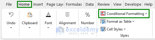
• Go to Home and select Conditional Formatting (in the Styles group).

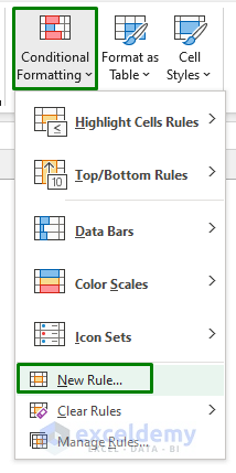
• Go to New Rule from the Conditional Formatting drop-down.

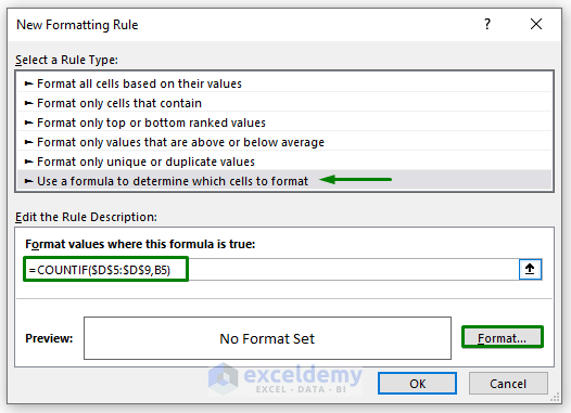
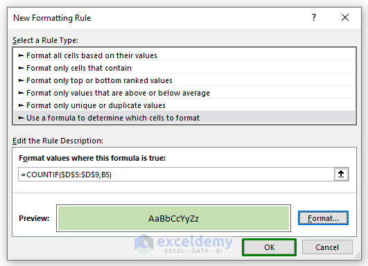
• The New Formatting Rule window will open. Choose the Rule Type: Use a formula to determine which cells to format.
• Insert the formula below in the field: Format values where this formula is true.

• Click on Format.

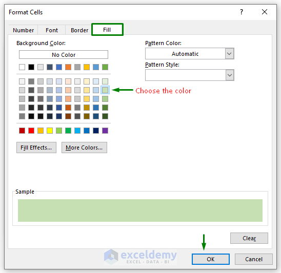
• Choose the highlight color from Fill and click OK.

• Click OK to close the dialog box.

• You will see all the cells containing text from the list Fruit 2 highlighted.

Method 2 – Apply the MATCH Function to Highlight Cells That Have Text from a List

Steps:

• Select the dataset (B5:C14).

• Go to Home, then to Conditional Formatting, and select New Rule.
• Choose the Rule Type: Use a formula to determine which cells to format.
• Use the following formula in the field: Format values where this formula is true.

• Click on the Format button and choose the highlight color from the Fill tab.
• Click OK twice to close the dialog boxes.

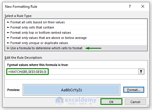
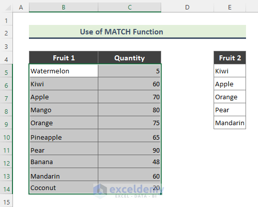
• All the cells containing text from the list Fruit 2 are highlighted in Fruit 1.

Read More: How to Highlight Selected Text in Excel

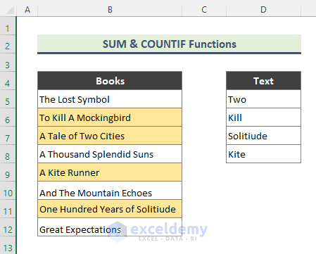
Method 3 – Combining SUM and COUNTIF Functions to Highlight Cells

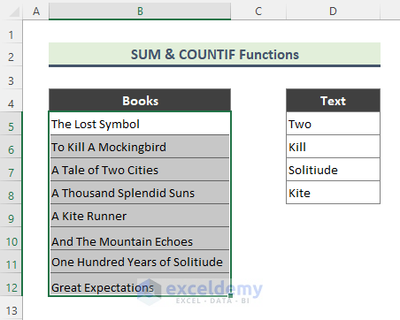
We have a dataset named Books (B4:B12), containing some book names. In another list Text (D5:D8), we have a list of single words. We will highlight the words of Text in dataset Books.

Steps:

• Select the dataset (B5:B12).

• Go to the Home tab and select Conditional Formatting drop-down.
• Select New Rule.
• The New Formatting Rule window will show up. Choose the Rule Type: Use a formula to determine which cells to format.
• Use the following formula in the field: Format values where this formula is true.

• Click on the Format button and select the highlight color from the Fill tab.
• Click OK twice to close the dialog boxes.

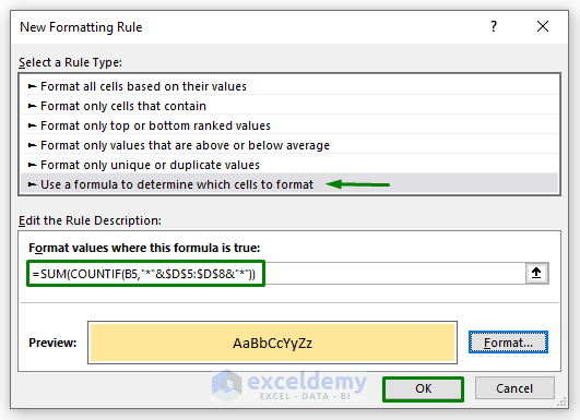
• Cells containing text from the list Text are highlighted in the Books.

Read More: How to Highlight Cells in Excel Based on Value

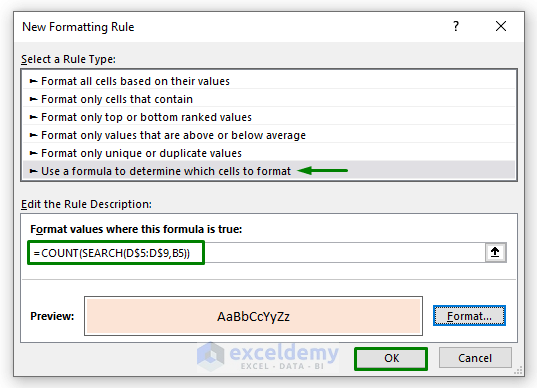
Method 4 – Use COUNT and SEARCH Functions to Highlight Cells That Contain Text from a List

Steps:

• Select the dataset (B5:B14).

• Go to Home, then to Conditional Formatting, and select New Rule.
• Choose the Rule Type: Use a formula to determine which cells to format.
• Use the following formula in the field: Format values where this formula is true.

• Click on the Format button and choose the highlight color from the Fill tab.
• Click OK twice to close the dialog boxes.

• Cells containing fruit names from the list Fruit 2 are highlighted in Fruit 1.

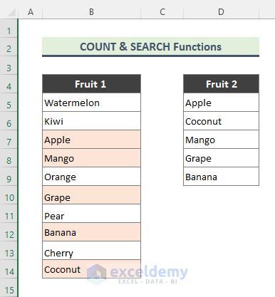
The SEARCH function counts the number of characters at which a specific character or text string is first found, reading left to right. The COUNT function counts the number of cells in a range that contains numbers.

Read More: How to Highlight Cells Based on Text in Excel

Method 5 – Apply a Formula and a Drop-Down List to Highlight Cells from a List

Steps:

• Create the drop-down list from some fruit names in cell D5. (Use the Data Validation option and insert the values manually or via a formula into the Source panel.)

• Select the dataset (B5:B14).

• Go to Home and select Conditional Formatting.
• Choose New Rule.
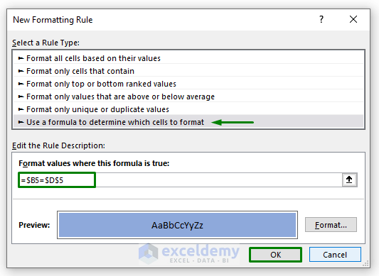
• The New Formatting Rule dialog will appear. Choose the Rule Type: Use a formula to determine which cells to format.
• Insert the following formula in the field: Format values where this formula is true.

• Click on the Format button and select the highlight color from the Fill tab.
• Click OK twice to close the dialog boxes.

• Cells containing fruits from the drop-down list are highlighted.

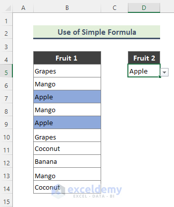
• If you change the fruit name from the drop-down, the highlighted cells change accordingly.

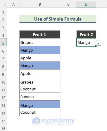
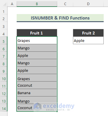
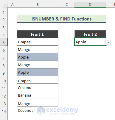
Method 6 – Excel ISNUMBER and FIND Functions to Highlight Cells from a List

Steps:

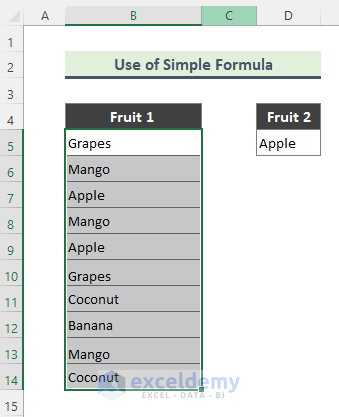
• Create the drop-down list from some fruit names in Cell D5.

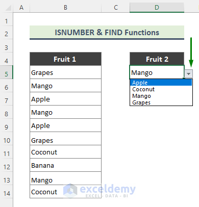
• Select the dataset (B5:B14).

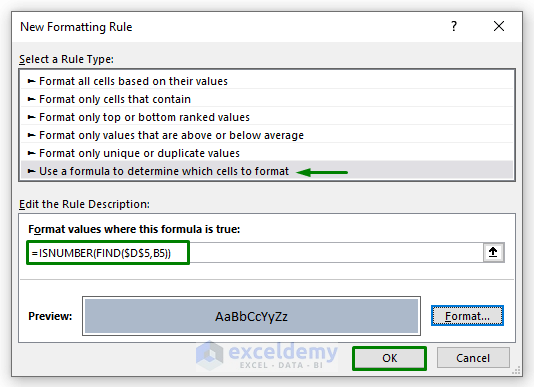
• Go to Conditional Formatting and choose New Rule.
• Choose the Rule Type: Use a formula to determine which cells to format.
• Insert the following formula in the field: Format values where this formula is true.

• Click on the Format button and choose the highlight color from the Fill tab.
• Click OK twice to close the dialog boxes.

• Here’s the result.

The FIND function returns the starting position of one text string within another text string (case-sensitive). The ISNUMBER function checks whether a value is a number and returns TRUE or FALSE.

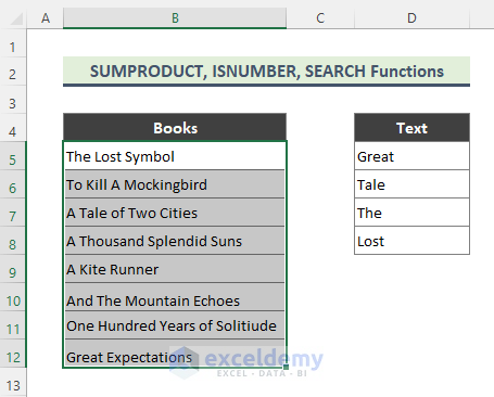
Method 7 – SUMPRODUCT, ISNUMBER, and SEARCH Function Combination to Highlight Cells That Contain Text from a List

Steps:

• Select the dataset (B5:B12).

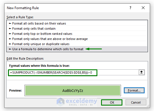
• Select New Rule from the Conditional Formatting drop-down.
• The New Formatting Rule dialog box will appear.
• Choose the Rule Type: Use a formula to determine which cells to format.
• Insert the following formula in the field: Format values where this formula is true.

• Click on the Format button and choose the highlight color from the Fill tab.
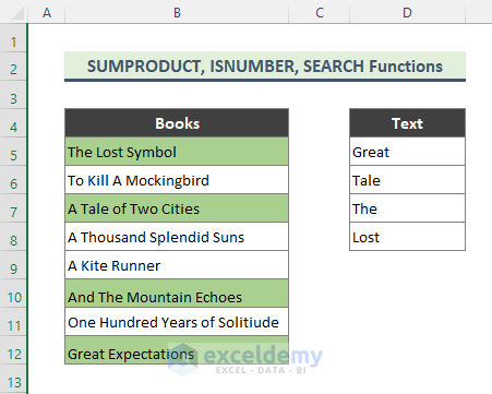
• Click OK twice to close the dialog boxes.

• Cells containing book names with the text from the list Text are highlighted.

How Does the Formula Work?

➤ SEARCH($D$5:$D$8,B5)

This part of the formula returns:

{#VALUE!;#VALUE!;1;5}

The SEARCH function returns the position of the value. But it returns an error (#VALUE!) if the value is not found.

➤ ISNUMBER(SEARCH($D$5:$D$8,B5))

The ISNUMBER function converts all error results to FALSE and other results to TRUE.

This part returns:

{FALSE;FALSE;TRUE;TRUE}

➤ –ISNUMBER(SEARCH($D$5:$D$8,B5))

This part returns:

{0;0;1;1}

The double minus (—) sign converts all FALSE and TRUE values to 0 and 1.

➤ SUMPRODUCT(–ISNUMBER(SEARCH($D$5:$D$8,B5)))>0

This part returns:

{TRUE;FALSE;TRUE;FALSE;FALSE;TRUE;FALSE;TRUE}

Finally, the SUMPRODUCT function tests the previous result against zero (0) and thus guides the Conditional Formatting rule to highlight cells.

Download the Practice Workbook

Related Articles

• How to Highlight Blank Cells with Conditional Formatting in Excel
• How to Highlight Cell If Value Is Less Than Another Cell in Excel
• How to Highlight Cells in Excel but Not Print
• Highlight Cell Using the If Statement in Excel

<< Go Back to Highlight Cell | Highlight in Excel | Learn Excel