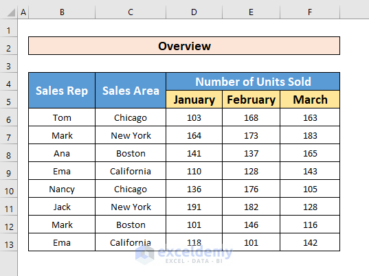
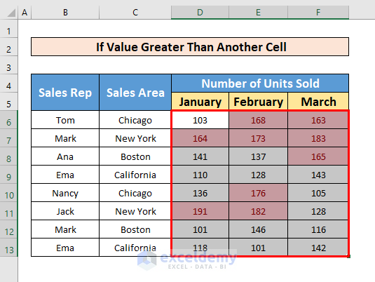
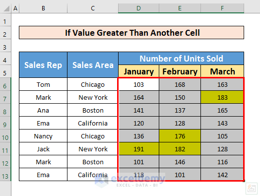
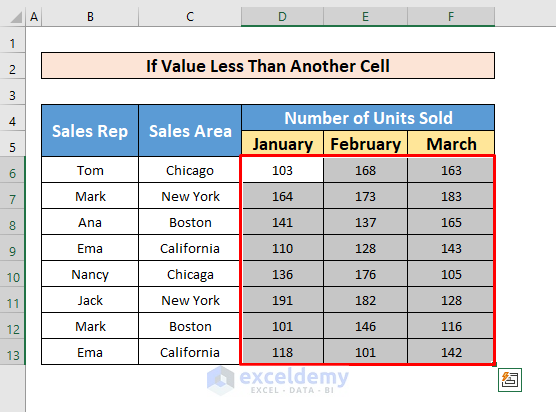
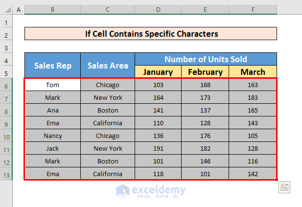
How to Highlight Cell Using the If Statement in Excel (7 Ways) -

Let’s say we have the following dataset: Sales Representative’s Name, their Sales Area, and the Number of Units Sold in each month of the first quarter, sorted in columns B, C, D, E, and F respectively. You can use the values in columns D, E, and F to highlight individual cells, rows, or columns. Here’s an overview of the dataset in the example, but you can change the values when trying out formula to see how it affects highlighting.

1. Apply Conditional Formatting to Highlight Cells with the If Statement

Conditional Formatting is a crucial tool in Excel to highlight cells. It minimizes the need to learn complex formulas and can be applied to different ranges seamlessly. There are several different options that the Conditional Formatting tool can use.

1.1 Highlight Cell Value Is Greater Than Another Cell

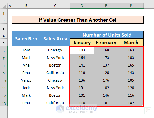
If you want to find out the sales where the number of units sold is more than 150, you can directly highlight the cells which have a value higher than 150. Follow these instructions to do so.

Step 1:

First, select the cell range.

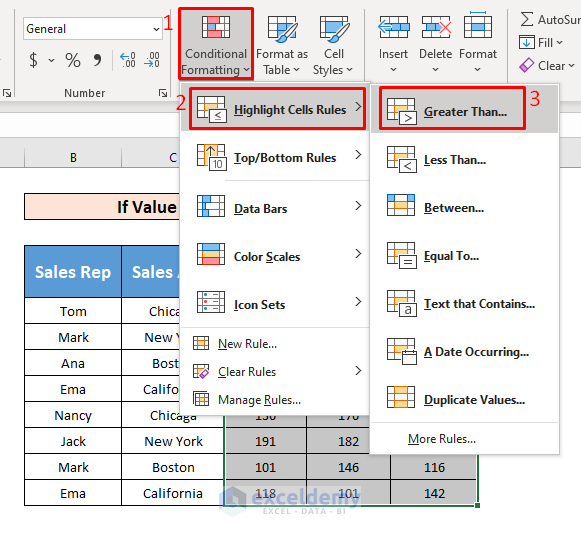
After selecting the cells, go to,

Home → Styles → Conditional Formatting → Highlight Cells Rules → Greater Than.

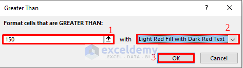
A window named Greater Than will pop up. In the Format cells that are GREATER THAN box, insert 150 as the cut-off value, and in the “with” box select the formatting style with which you want to highlight the cells. The default highlighter value is Light Red Fill with Dark Red Text. Then, click OK.

After clicking on the OK button, cells with a value greater than 150 will be automatically highlighted.

You can also highlight cells by applying the COUNTIF function. To do that, follow step 2 below.

Step 2:

Select cells D6 to F13, then go to Conditional Formatting and select New Rule.
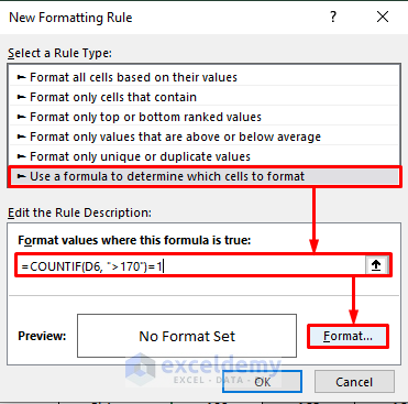
A window named New Formatting Rule should pop up.
Under Select a Rule Type, pick Use a formula to determine which cells to format.
Next, type the COUNTIF function in the Format values where this formula is true box. The COUNTIF function is

=COUNTIF(D6, ">170")=1

Then, to give cells format, click on the Format box.

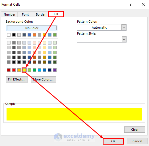
A Format Cells window will appear in front of you. From that window, select the Fill menu and then choose a color (such as the default yellow) from the Background Color selector. Press OK to confirm.

After that, again press OK.

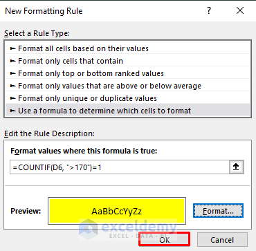
Finally, the conditional formatting will run the COUNTIF function through the entire cell range and highlight cells with values over 170.

1.2 Highlight Cell If Value Is Equal to Another Cell

You can also use Conditional Formatting for highlighting cells with a precise value. To highlight cells whose value is equal to 136, follow the steps below.

Steps:

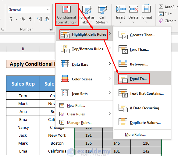
First of all, select the cells array D6 to F13, and then, from your Home Tab, go to,

Home → Styles → Conditional Formatting → Highlight Cells Rules → Equal To

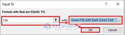
When you press on the Equal To option, an Equal To window pops up.
Now, in the Format cells that are Equal To box insert 136 as the cut-off value, and in the with box select Green Fill with Dark Green Text to highlight cells. At last, click on OK.

By clicking on the OK box, you will be able to highlight cells whose value is equal to 136.

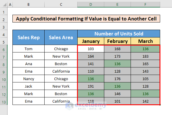
You can swap out the exact value in the formula with a fixed cell reference like “$B$6” to highlight all cells that have the same value as the reference (including the cell itself).

1.3 Highlight Cell If Value Is Less Than Another Cell in Excel

You can also learn how to highlight cells whose value is less than another cell by using Conditional Formatting. Follow the instructions below to highlight cells with a value lower than 125.

Steps:

Select cells D6 to F13.

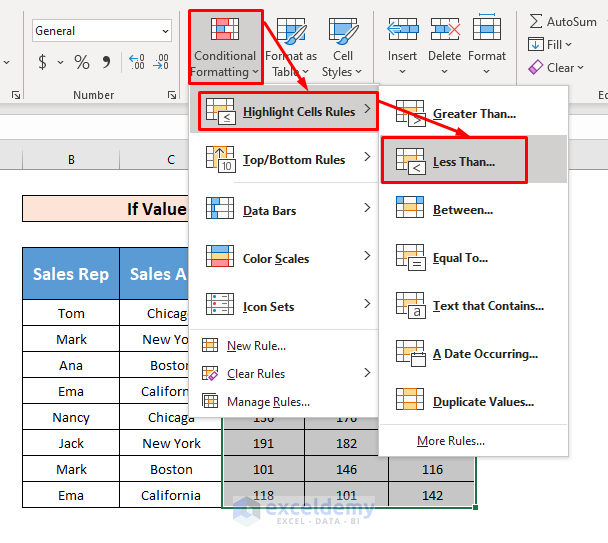
In the Home Tab, go to,

Home → Styles → Conditional Formatting → Highlight Cells Rules → Less Than

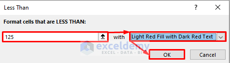
A window named Less Than will appear. Now, in the Format cells that are Less THAN box, insert 125 as the cut-off value, and in the with box select the Light Red Fill with Dark Red Text formatting (or whatever highlighting you want) to highlight cells. Hit OK.

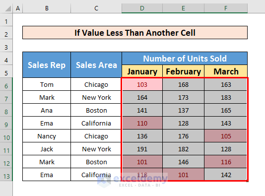
Finally, you will see the cells that have a value of less than 125 are highlighted.

1.4 Highlight Cell If Cell Contains Specific Characters in Excel

You can also conditional formatting to highlight cells with specific characters. Use the instructions below to get a highlight of cells containing “New York” somewhere in its value.

Steps:

Select the cells B6 to F13.

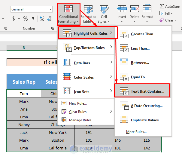
From your Home Tab, go to,

Home → Styles → Conditional Formatting → Highlight Cells Rules → Text that Contains

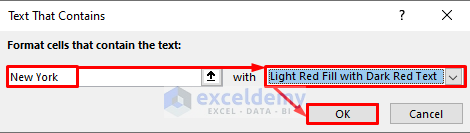
A Text that Contains window will pop up. Now, in the Format cells that contain the text box, insert “New York” as the specific string value, and in the with box select the formatting style with which you want to highlight the cells. The stock value is Light Red Fill with Dark Red Text. Click on OK to continue.

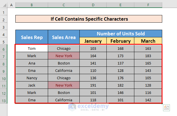
After completing the above process, Excel will highlight cells that contain New York. Note that a cell which contains additional text will also be highlighted.

1.5 Highlight Cell If Cell Contains Duplicate or Unique Value

You can also use conditional formatting to highlight cells with duplicate values or cells with unique values. To do that, please follow the instructions below.

Steps:

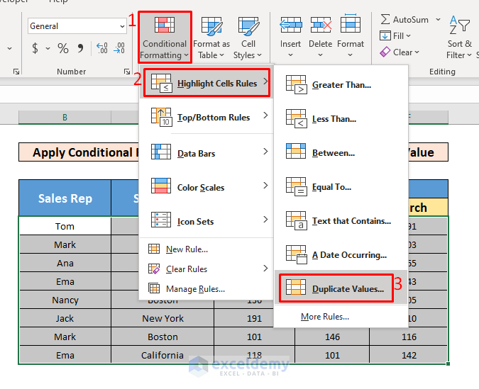
First, select your entire dataset. Then, from your Home Tab, go to,

Home → Styles → Conditional Formatting → Highlight Cells Rules → Duplicate Values

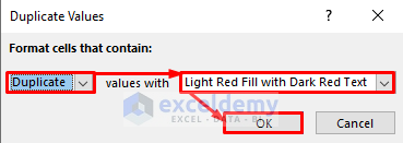
After that select Duplicate from the box Format cells that contain and then select Light Red Fill with Dark Red Text for the formatting style in the values with, at last, press OK.

Here’s how a sample table will look with all duplicate values highlighted.

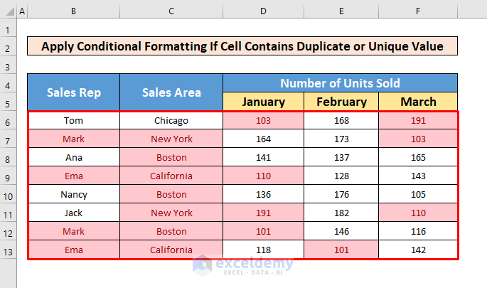
To select cells with unique values, choose the “Unique” option instead “Duplicate” in the “Duplicate Values” box. In the previous sample, the resulting cell highlighting will essentially be reversed.

1.6 Highlight Cell If Cell Does Not Have Value in Excel

Suppose there are some blank cells in a large dataset, and you want to highlight them for greater visibility. To highlight the blank cells using Conditional Formatting, follow the steps below for the example dataset:

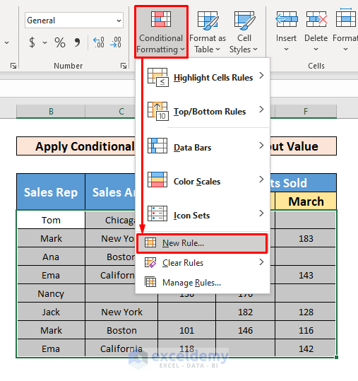
First of all, select cells B6 to F13 from our dataset and then go to,

Home → Conditional Formatting → New Rule

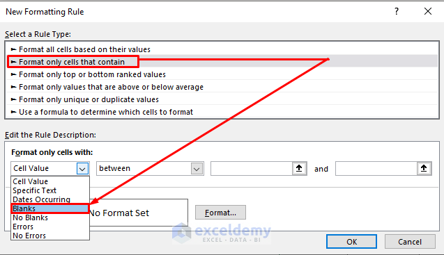
The New Formatting Rule window will appear. Under Select a Rule Type, choose Format only cells that contain.
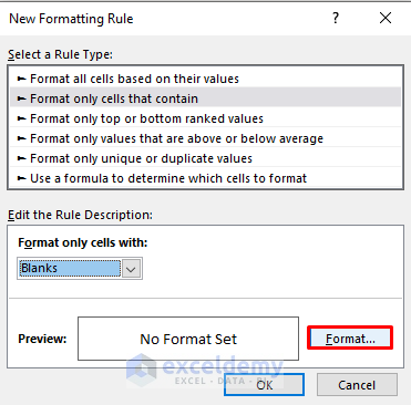
In the Format only cells with dropdown, select “Blanks.”

Now, press on the Format box.

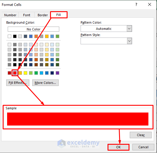
After that, a Format Cells window will appear in front of you.
Go to the Fill tab and select a color from the Background Color. Then, press OK to confirm the formatting.

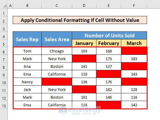
Select OK again in the New Formatting Rule window to finalize the formula.

After completing the above process, Excel will highlight cells without a value.

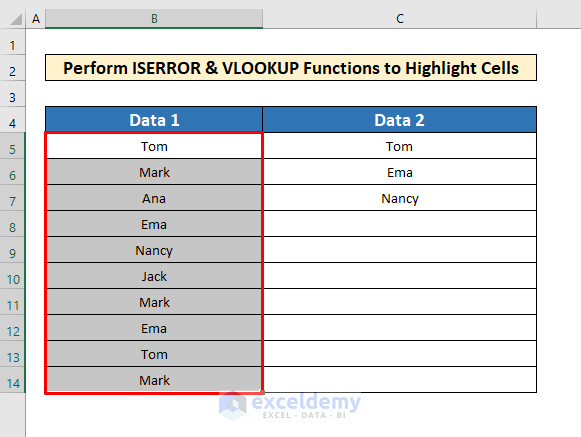
2. Perform the ISERROR and VLOOKUP Functions to Highlight Cell with If Statement

You can apply the ISERROR and VLOOKUP functions to highlight cells that contain values in a range.

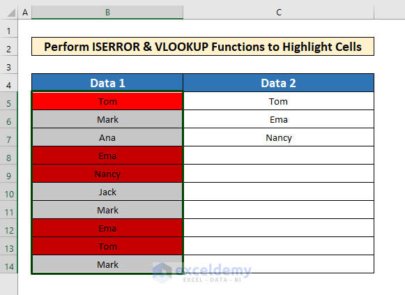
Let’s say there’s a dataset with some arbitrary names and you need to highlight the names in column B that can be found in column C. Follow the instructions below to do so:

First, select cells B5 to B14.

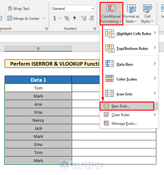
Now, from your Home Tab, go to,

Home → Conditional Formatting → New Rule

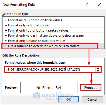
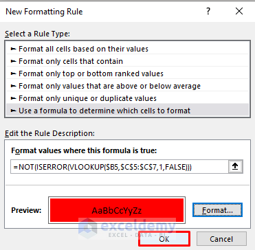
After that, a New Formatting Rule window will appear. Firstly, select Use a formula to determine which cells to format from Select a Rule Type. Secondly, type the formula in the Format values where this formula is true box. The formula is:

=NOT(ISERROR(VLOOKUP($B5, $C$5:$C$7, 1, FALSE)))

Then select the Format box.

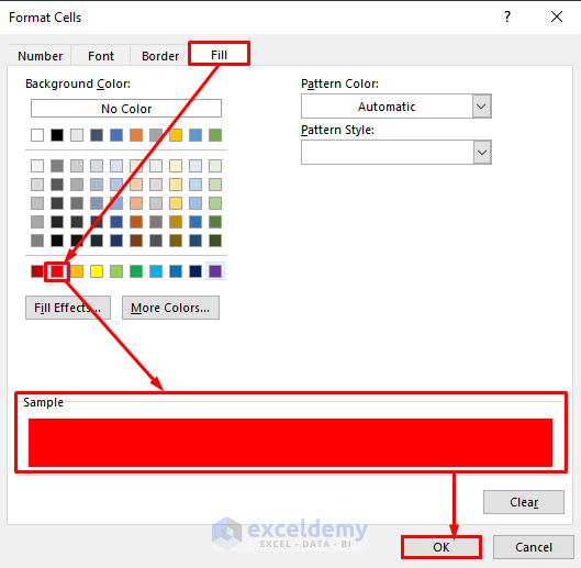
A Format Cells window will appear in front of you.
Go to the Fill tab and choose a color from the Background Color selector, such as the recommended Red. To finalize the formatting, press OK.

Back in the New Formatting Rule window, press OK.

Finally, Excel will highlight the cells containing values that can be found in column C.

Things to Remember

There is no error when the ISERROR Formula returns FALSE if the value is found.

The NOT Function reverses the ISERROR Formula’s return, thus FALSE returns TRUE.

How to Highlight Cell Using the If Statement in Excel (7 Ways)

1. Apply Conditional Formatting to Highlight Cells with the If Statement

1.1 Highlight Cell Value Is Greater Than Another Cell

1.2 Highlight Cell If Value Is Equal to Another Cell

1.3 Highlight Cell If Value Is Less Than Another Cell in Excel

1.4 Highlight Cell If Cell Contains Specific Characters in Excel

1.5 Highlight Cell If Cell Contains Duplicate or Unique Value

1.6 Highlight Cell If Cell Does Not Have Value in Excel

2. Perform the ISERROR and VLOOKUP Functions to Highlight Cell with If Statement

Things to Remember

Related Articles

Leave a reply Cancel reply