How to Highlight Cells Based on Text in Excel (2 Methods)

Highlighting cells with specific text in MS Excel is useful for easily finding matching text in datasets.

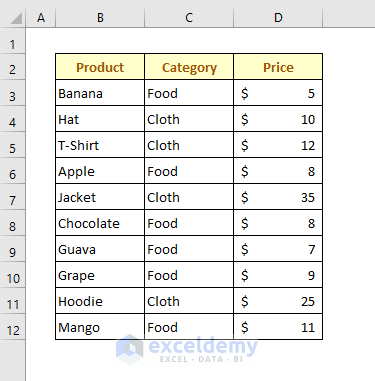
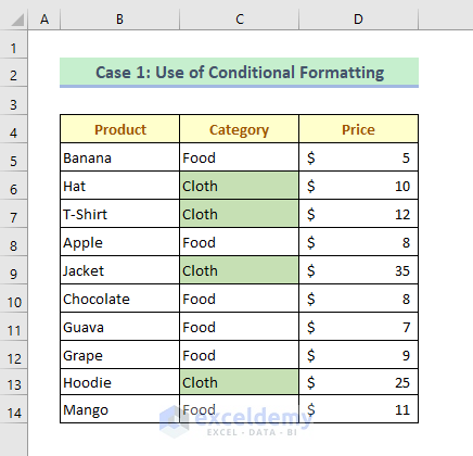
Our sample dataset contains a list of food and clothing items with their prices.

Sample Dataset: How to Highlight Cells Based on Text in Excel

Method 1 – Using Excel Conditional Formatting to Highlight Cells Based on Text Value

Conditional formatting will help you to highlight cells with a certain color, depending on the cell’s values, text, and conditions.

1.1. Use of New Rule from the Conditional Formatting

The New Rule option provides you with the option to use any suitable self-made formula for your dataset.

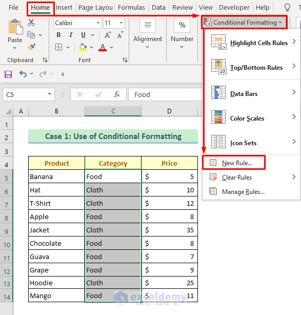
Step 1:

⏩ Go to Home > Conditional Formatting > New Rule.

A dialog box will appear.

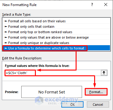
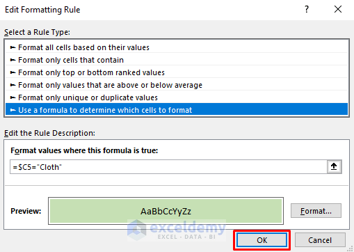
Excel Conditional Formatting to Highlight Cells Based on Text Value: Select New Rule

Step 2:

⏩ Select Use a formula to determine which cells to format from the Select a Rule Type drop-down.

⏩ Type the following formula in Format values where this formula is true box.

=$C5="Cloth"

⏩ Click the Format option.

Another dialog box named “Format Cells” will open up.

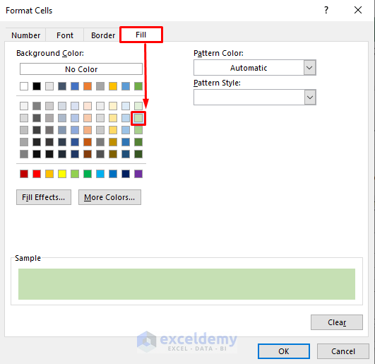
Create New Rule in Conditional Formatting to Highlight Cells Based on Text Value

Step 3:

⏩ Choose your desired color from the Fill tab. I have chosen a light green color.

⏩ Press the OK and it will go back to the previous dialog box.

Fill the highlighted cells with color

Step 4:

⏩ Press OK.

The cloth items are highlighted with the chosen color.

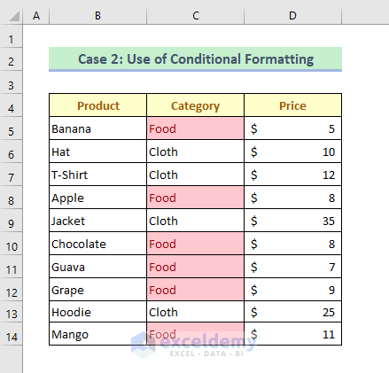
Output: New Rule from Conditional Formatting in Excel to highlight cells based on text value

1.2. Using “Text That Contains…” Feature from the Conditional Formatting

This method works with both whole and partial text.

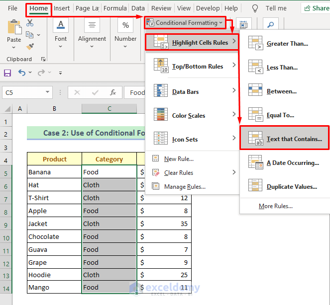
Step 1:

⏩ Go to Home > Conditional Formatting > Highlight Cells Rules > Text that Contains.

A dialog box will open.

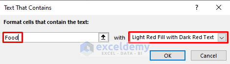
Conditional Formatting to Highlight Cells Based on Text Value

Step 2:

⏩ Type Food in the Format cells that contain the text bar.

⏩ Select your desired highlight color, and press OK.

Conditional Formatting to Highlight Cells Based on Text Value

The food items are highlighted.

Conditional Formatting to Highlight Cells Based on Text Value

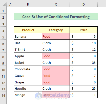
1.3. Applying “Equal To…” Option from the Cell Rules for Highlighting

This method only works with whole text in a cell; it’s not applicable for partial text.

Step 1:

⏩ Go to Home > Conditional Formatting > Highlight Cells Rules > Equal To

A dialog box will open up.

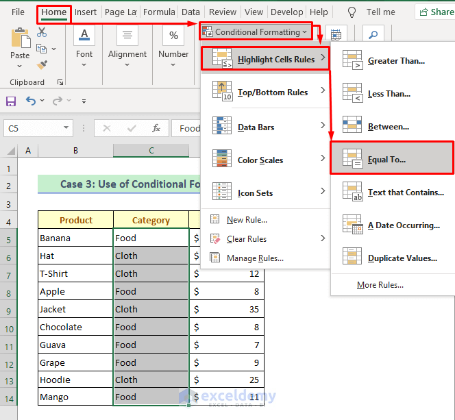
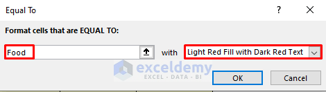
Conditional Formatting to Highlight Cells Based on Text Value

Step 2:

⏩ Type Food in the Format cells that are EQUAL TO box.

⏩ Pick your desired highlight color.

⏩ Press OK.

Conditional Formatting to Highlight Cells Based on Text Value

All the cells with food items are highlighted.

Conditional Formatting to Highlight Cells Based on Text Value

Method 2 – Combining ISNUMBER & SEARCH Functions to Highlight Cells Based on Text Value in Excel

In this method, we’ll use the combination of two functions to highlight cells in a different way. Those are the ISNUMBER function and the SEARCH function. Instead of using color, we’ll highlight with a remark here. If specified text is found, then it will show TRUE, and if not, then it will show FALSE. A new column has been added to the sample dataset for showing remarks. We’ll do it here for food items.

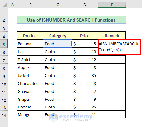
Step 1:

⏩ Type this formula in cell E5–

=ISNUMBER(SEARCH("Food",C5))

⏩ Hit the Enter key.

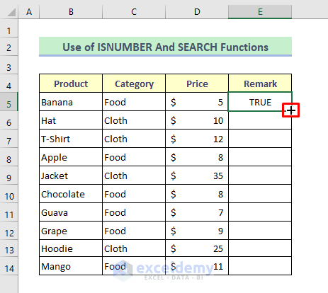
Conditional Formatting to Highlight Cells Based on Text Value

Double-click the Fill Handle icon to copy the formula over the rest of the cells.

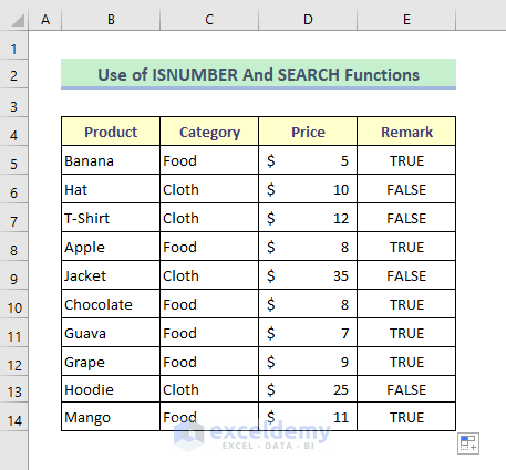
Here’s our output.

⏬ Formula Breakdown:

⏩ SEARCH(“Food”,C5)

The SEARCH function will return the position of the text “Food” in cell C5; if the text is not found, then it will show #VALUE!. So, it will return as:

⏩ ISNUMBER(SEARCH(“Food”,C5))

The ISNUMBER function will return TRUE if it gets any number and return FALSE if it gets #VALUE!. It will return for cell C5–

TRUE

Download Sample Excel Workbook

Highlight Cells Based on Text.xlsx