While working with a dataset in an Excel file, it is very normal that some cells may remain blank. If you apply any formula referring to the blank cells, it may hinder your work and result in errors. If you want to avoid these problems, then highlighting the blank cells could be one of the best solutions. In this case, Conditional Formatting will pave the way for highlighting the blank cells in your Excel file. In this article, I will show you how to highlight blank cells with conditional formatting in Excel.
Highlight Blank Cells with Conditional Formatting in Excel: 2 Ways
There are several ways to check if a cell is empty or not. In this section, you will find 2 easy and effective ways to highlight blank cells with conditional formatting in Excel. I will demonstrate them one by one here. Let’s check them now!
1. Format Blank Cells with Conditional Formatting
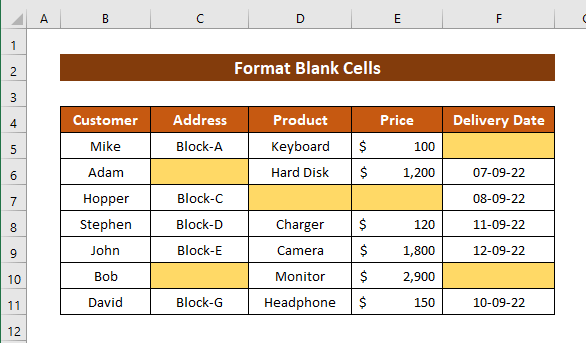
Let’s say we have got a dataset of some customers’ information: their Address, ordered Products, Price, Delivery Date, etc.
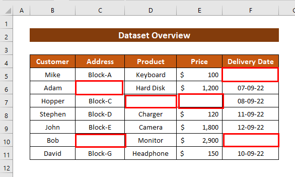
You can see that all the cells don’t contain data. Some cells are blank in the dataset. We want to highlight these blank cells with Conditional Formatting. In order to demonstrate this method, proceed with the following steps.
💡 Steps:
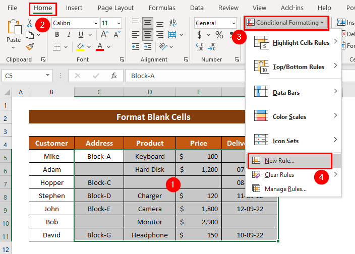
- First of all, select the range of the data> go to the Home tab> click Conditional Formatting> select New Rule.
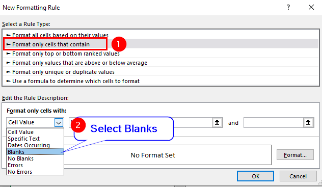
- Then, the New Formatting Rule dialogue box will show up.
- Here, click Format only cells that contain in the Select a Rule Type field and choose Blanks from the dropdown of the Format only cells with field.
- Now, click Format.
![]()
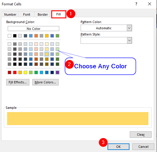
- After that, the Format cells common box will appear.
- Here, from the Fill icon, choose a color type and click OK to close the command box.
- Now, closing this box will return you to the New Formatting Rule dialogue box. Click OK to close this box also.
![]()
- Hence, your blank cells will be highlighted with the color format you have chosen.
Read More: How to Highlight Selected Cells in Excel
2. Highlight Blank Cells Applying Conditional Formatting with Formula
For our same set of data, we will again apply Conditional Formatting to highlight the blank cells. For the previous method, we have applied the format for blank cells. Now, we will apply the Conditional Formatting Formula to highlight blank cells. Let’s follow the steps with proper illustrations.
💡 Steps:
- Firstly, select the data range> go to the Home tab> click Conditional Formatting> select New Rule.
![]()
- Then, the New Formatting Rule dialogue box will show up.
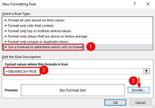
- Here, click Use a formula to determine which cells to format in the Select a Rule Type field and apply the following formula to the Format values where this formula is true field.
=ISBLANK(C5)=TRUE
- Now, click Format.
- After that, the Format cells common box will appear.
- Here, from the Fill icon, choose a color type and click OK to close the command box.
![]()
- Again, click OK to close the New Formatting Rule dialogue box.
![]()
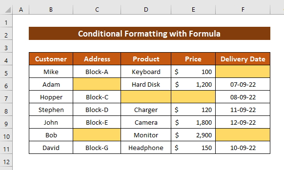
- As a result, the cells that are blank will be highlighted with the selected color.
Read More: How to Highlight Cell If Value Is Less Than Another Cell in Excel
How to Remove Conditional Formatting
As you can apply Conditional Formatting to a cell, Excel also allows you to remove the formatting you have applied. Here, we will learn different methods for removing Conditional Formatting.
1. Remove Conditional Formatting Keeping Blank Cells Highlighted
Previously we have shown you the application of Conditional Formatting to highlight the blank cells. Let’s say you want to remove the formatting but still want to keep the blank cells highlighted. Don’t worry, Excel is with you!
In order to do so, just proceed with the steps below.
💡 Steps:
- First of all, select the whole dataset and click the cell where you want the dataset after removing the format.
- Then, click the Clipboard icon from the Home tab.
![]()
- Now, on the left side of the Excel window, the copied item will appear. Click on this.
![]()
- Now, your selected dataset will be pasted in the cell that you have clicked at first.
- Now, delete the columns that contain the Conditionally Formatted dataset.
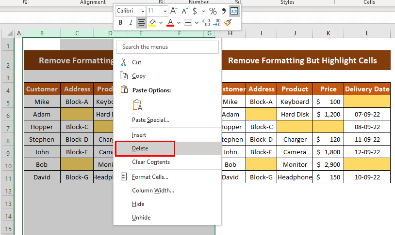
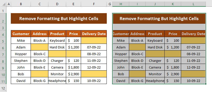
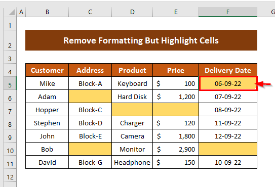
- Hence, your newly pasted data will be repositioned.
![]()
- You can check whether Conditional Formatting is removed or not by entering some text into a blank cell. If the formatting is removed, the cell won’t change the color.
2. Undo Conditional Formatting by Clearing Rules
You can also remove the Conditional Formatting without keeping the cell highlighted. In this case, you have to clear the rules.
💡 Steps:
- Here, select the cells of the data range, and the Quick Analysis tool will appear at the right end of the selected data. Click on it.
- Now, click Clear from the formatting icon.

- Hence, the cells will clear the formatting totally. It won’t keep the highlighted cells anymore and make the dataset just like it was before formatting.
![]()
Download Practice Workbook
You can download the practice book from the link below.
Conclusion
In this article, I have tried to show you some methods to highlight blank cells with conditional formatting in Excel. I hope this article has shed some light on your way of this. Thanks for reading the article! If you have better methods, questions, or feedback regarding this article, please don’t forget to share them in the comment box. For more queries, kindly visit our website. Keep learning. Happy Excel! 🙂
Related Articles
- How to Highlight Cells in Excel but Not Print
- Cells Are Not Highlighting in Excel Formula
- How to Highlight Cells in Excel Based on Value
- How to Click One Cell and Highlight Another in Excel
- How to Highlight Cells Based on Text in Excel
- Highlight Cells That Contain Text from a List in Excel
- How to Highlight Cell Using the If Statement in Excel
<< Go Back to Highlight Cell | Highlight in Excel | Learn Excel
Get FREE Advanced Excel Exercises with Solutions!
