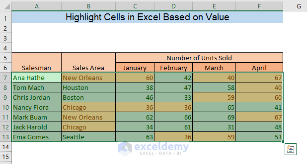
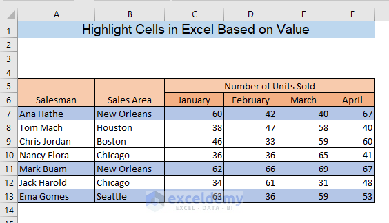
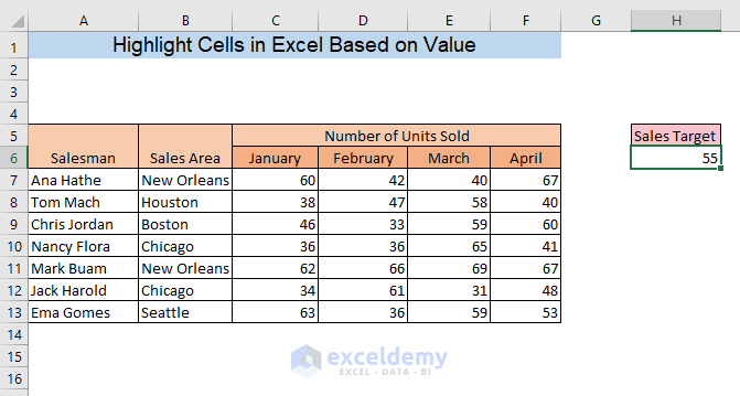
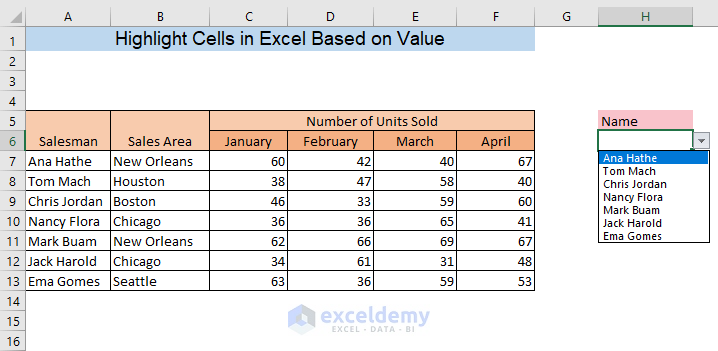
Let’s say we have a dataset where sales area and Number of units sold in different months of the first quarter by different salesmen are given. Now we will highlight cells based on different conditions of their value.
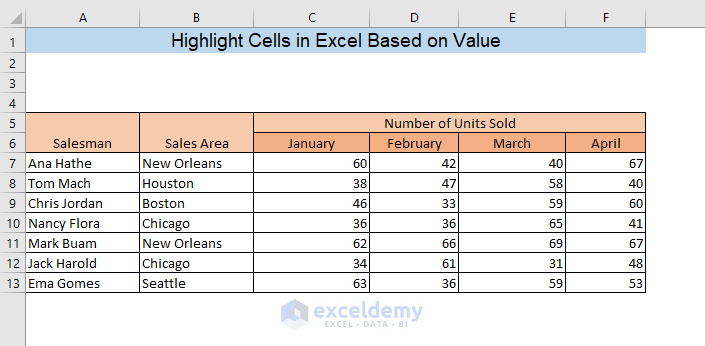
How to Highlight Cells in Excel based on Value: 9 Methods
Method 1 – Highlight Cells Above a Specific Values
Suppose we want to find out the sales where the number of units sold is more than 60.
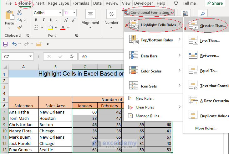
- Select the cells that have values.
- Go to Home > Conditional Formatting > Highlight Cells Rules > Greater Than.
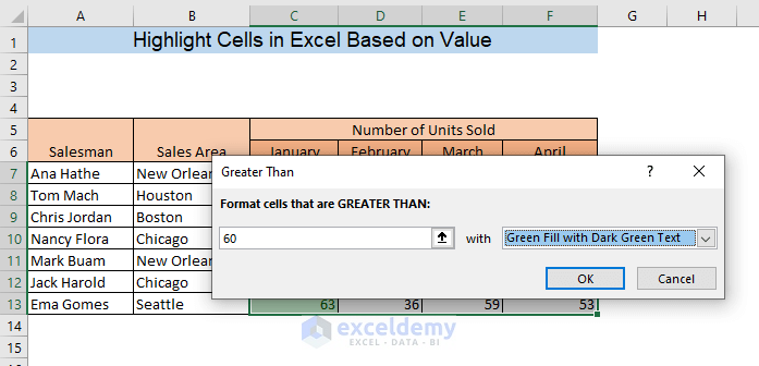
- After that, a window named Greater Than will appear.
- In the Format cells that are GREATER THAN box, insert the cut-off value.
- In the with box, select the formatting style with which you want to highlight the cells. We’ve selected Green Fill with Dark Green Text here.
- Click OK.
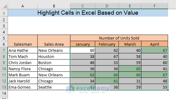
Now you will see the cells which have a value greater than 60 are highlighted.
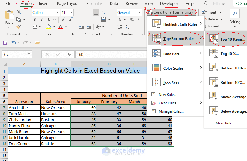
Method 2 – Highlight Top X Values
We will highlight the top ten values of our dataset.
- Select the cells with values you need to highlight.
- Go to Home > Conditional Formatting > Top/Bottom Rules > Top 10 Items.
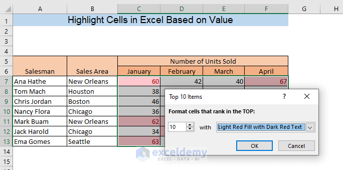
- After that, a window named Top 10 Items will appear.
- In the Format cells that rank in the TOP box, insert a number. It is 10 by default. The number determines how many highest-value cells will be highlighted.
- In the with box, select the formatting style with which you want to highlight the cells.
- Click OK.
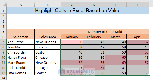
Now you will see the cells with the top ten values highlighted.
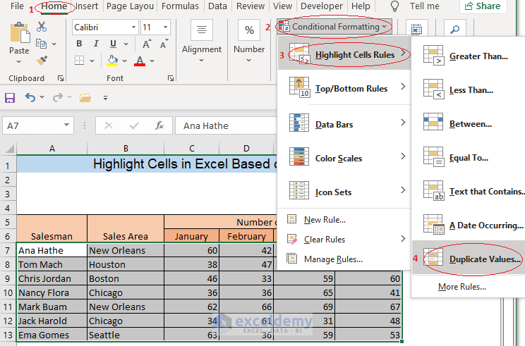
Method 3 – Format Duplicate or Unique Values
- Select your entire dataset.
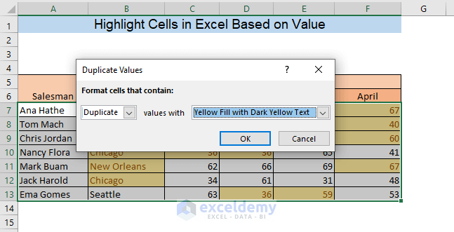
- Go to Home > Conditional Formatting > Highlight Cells Rules > Duplicate Values.
- To highlight the duplicate values, select Duplicate from the box Format cells that contain.
- Select the formatting style in the box values with. For this example, we’ve selected Yellow Fill with Dark Yellow Text.
- To highlight the unique values, select Unique from the box Format cells that contain.
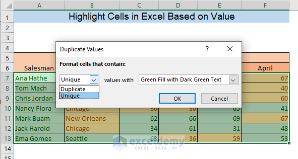
As a result, all the duplicate values will be highlighted with yellow fill with dark yellow text, and unique values will be highlighted with green fill with dark green text.
Read More: How to Highlight Selected Cells in Excel
Method 4 – Highlight Value Based on Multiple Criteria
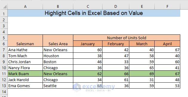
Suppose we want to find out the names of the salesmen who operate in New Orleans and sell more than 60 units every month of the first quarter.
- Select your dataset.
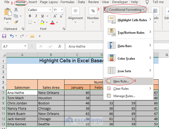
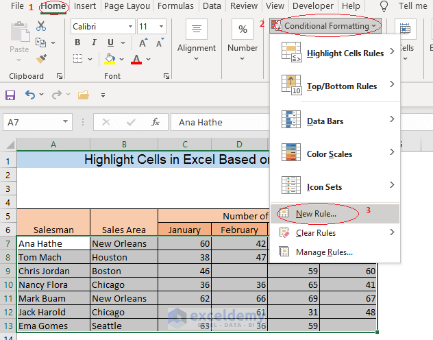
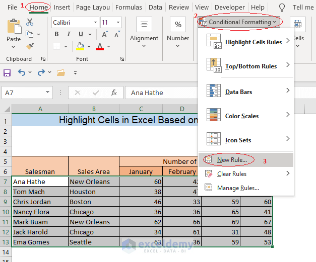
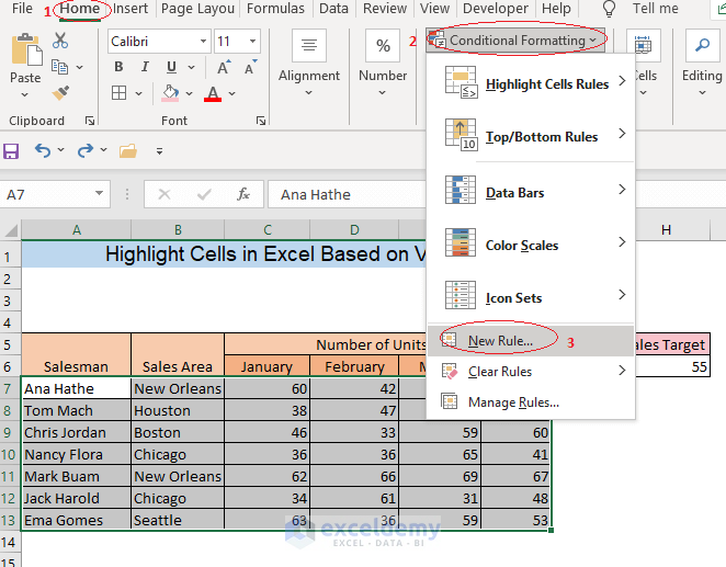
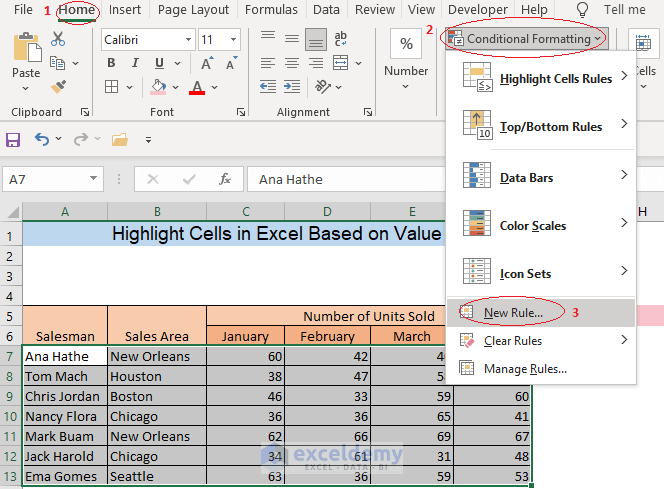
- Go to Home > Conditional Formatting > New Rule.
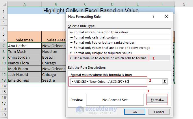
- New Formatting Rule window will appear. Select Use a formula to determine which cells to format from Select a Rule Type.
- Type the following formula in the Format values where this formula is true box:
=AND($B7="New Orleans",$C7:$F7>50)Here, the AND function will find out the cells that fulfil both criteria. $B7=”New Orleans” is the first criteria and $C7:$E7>50 is the second criteria where $C7:$E7 is the data range.
- Click on Format to select the formatting style.
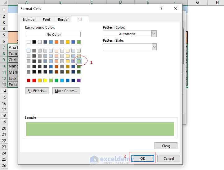
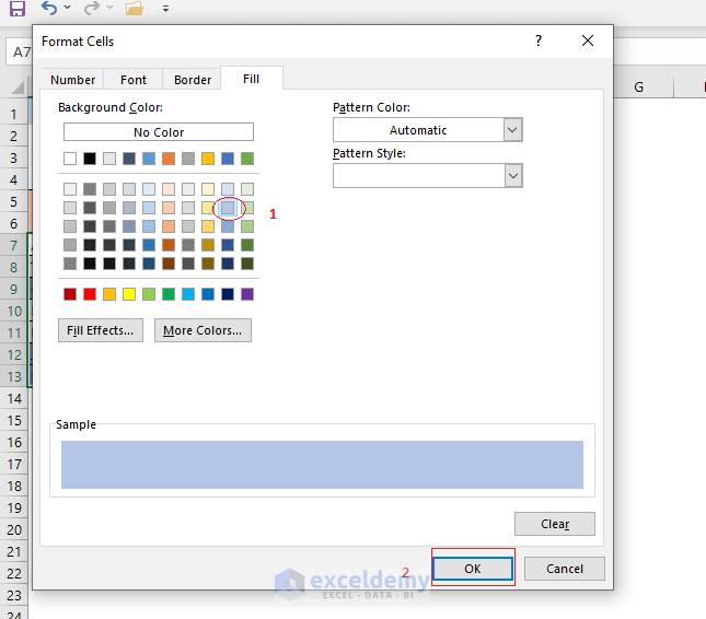
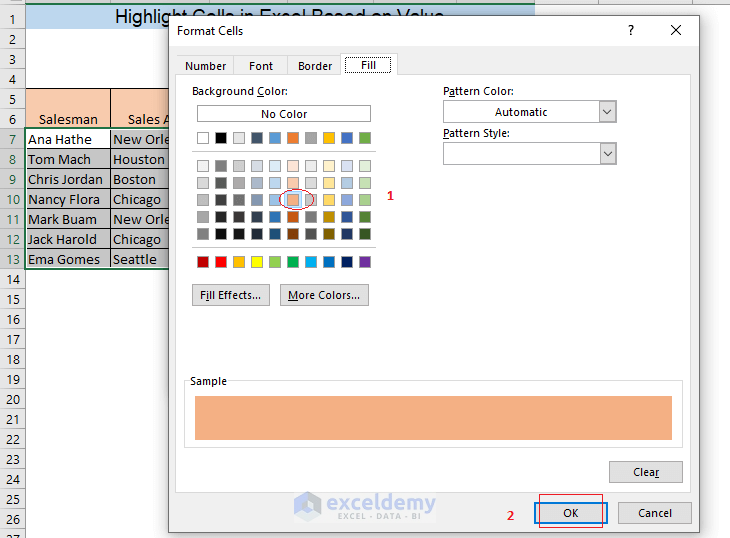
- In the Format Cells window, from the Fill tab, select the color with which you want to highlight the cells. Go to the other tabs for more customization.
- After selecting your preferred formatting, click on OK.
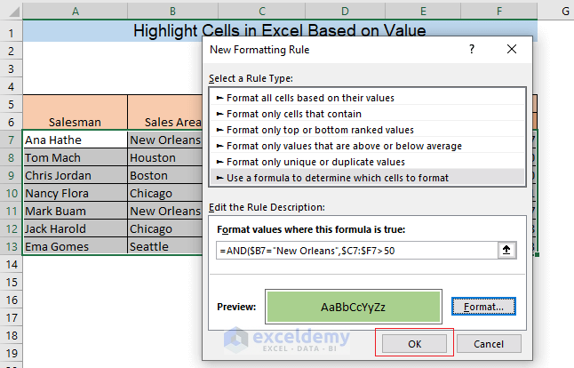
- You will see your formatting style in the preview box of the New Formatting Rule window. Click on OK.
The row with a matching value with the criteria is highlighted.
Method 5 – Highlight Rows which Contain Cells Without Value
- Select your entire dataset and go to Home > Conditional Formatting > New Rule.
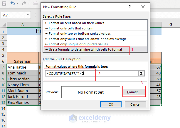
- New Formatting Rule window will appear. Select Use a formula to determine which cells to format from Select a Rule Type.
- Type the following formula in the Format values where this formula is true box:
=COUNTIF($A7:$F7,"")>0Here, the COUNTIF function will count the cells that are empty in the cell range $A7:$F7. If the number of empty cells is greater than zero in any particular row, the row will be highlighted.
- Click on Format to select the formatting style.
- After selecting your preferred formatting, click on OK.

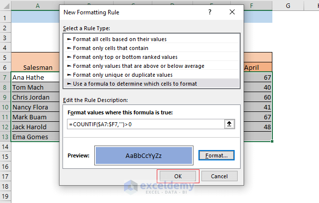
- You will see your formatting styles in the preview box of the New Formatting Rule window.
- Click on OK.
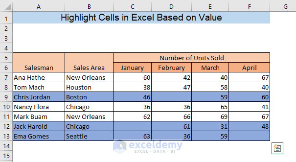
- The rows with blank cells are highlighted.
Read More: How to Highlight Blank Cells with Conditional Formatting in Excel
Method 6 – Create a Custom Conditional Formatting Rules to Highlight Values
Suppose we want to find out the salesmen who have sold more than 200 units in the first quarter.
- Select your dataset and go to Home > Conditional Formatting > New Rule.
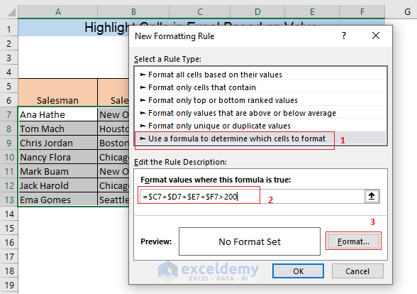
- New Formatting Rule window will appear. Select Use a formula to determine which cells to format from Select a Rule Type.
- Type the following formula in the Format values where this formula is true box:
=$C7+$D7+$E7+$F7>200Here, the formula will find out the rows where the total first-quarter sales are more than 200 units.
- Click on Format to select the formatting style.
- After selecting your preferred formatting from the Format cells box, click on OK.
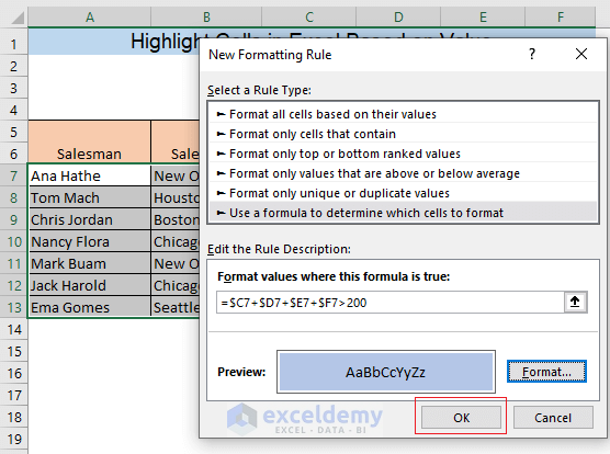
- You will see your formatting style in the preview box of the New Formatting Rule window.
- Click on OK.
- The rows where total first-quarter sales are more than 200 units highlighted.
Method 7 – Apply Conditional Formatting to Text
Suppose we want to find out how many salesmen are operating in Chicago.
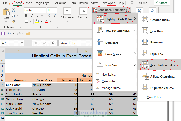
- Select all the cells of your dataset and go to Home > Conditional Formatting > Highlight Cells Rules > Text that Contains.
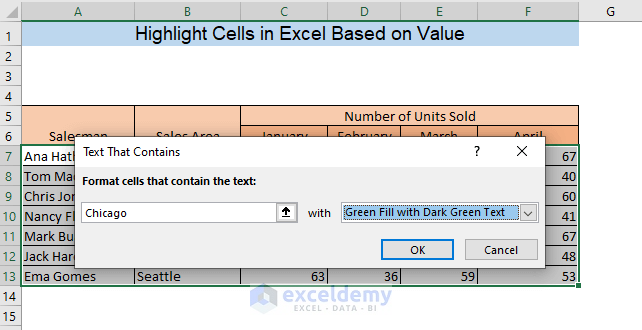
- A window named Text That Contains will appear. In the box Format cells that contain the text, type the text you want to find out: Chicago.
- Select your preferred formatting styles and press on OK.
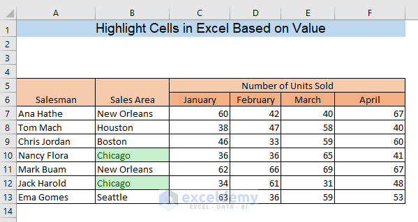
As a result, all the cells which contain the text Chicago will be highlighted.
Read More: How to Highlight Cells Based on Text in Excel
Method 8 – Highlight Cells Based on The Value of Another Cell
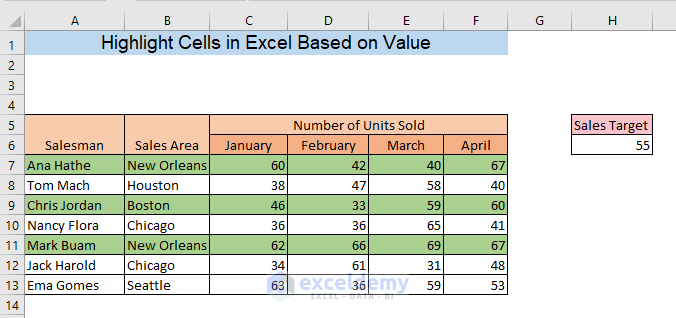
Let’s say for our dataset, there is a sales target in a month, which is inserted in cell H6.
- Select your dataset and go to Home > Conditional Formatting > New Rule.
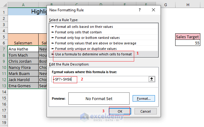
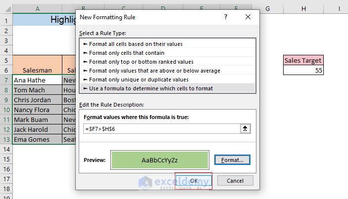
- New Formatting Rule window will appear. Select Use a formula to determine which cells to format from Select a Rule Type.
- Type the following formula in the Format values where this formula is true box:
=$F7>$H$6Here, the formula will find the cells of column F which have a higher value than cell H6.
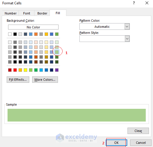
- Press Format to select a formatting style.
- After selecting your preferred formatting color from the Format cells box, click on OK.
- Your formatting style is in the preview box of the New Formatting Rule window.
- Click on OK.
You will get the rows highlighted where the cells of the F column have higher values than the value of cell H6.
Method 9 – Highlight Cells Based on Drop Down Selection
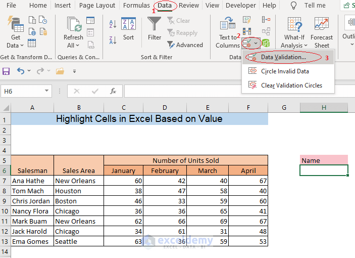
- Go to the Data Tools ribbon from the Data tab.
- Click on the icon on Data Validation to expand it and select Data Validation from the menu.
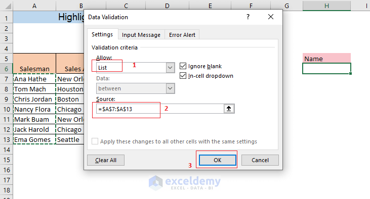
- The Data Validation window will open. Select List from the Allow: box.
- You will see a box named Source: will appear in the same window. Insert your data range in this box.
- Click on OK.
- A drop-down menu will be created in cell H6. If you click on the downward arrow beside this cell, you will see the list of the salesmen.
- Select your data and go to Home > Conditional Formatting > New Rule.
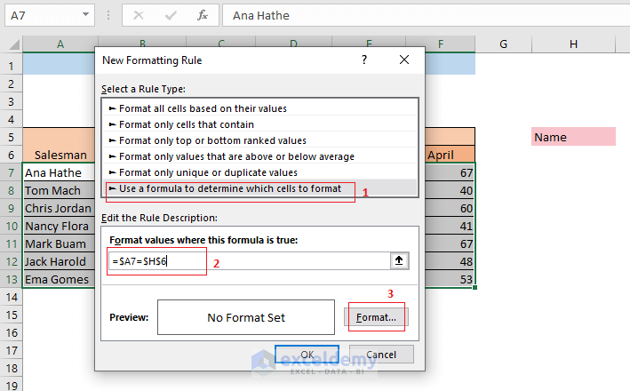
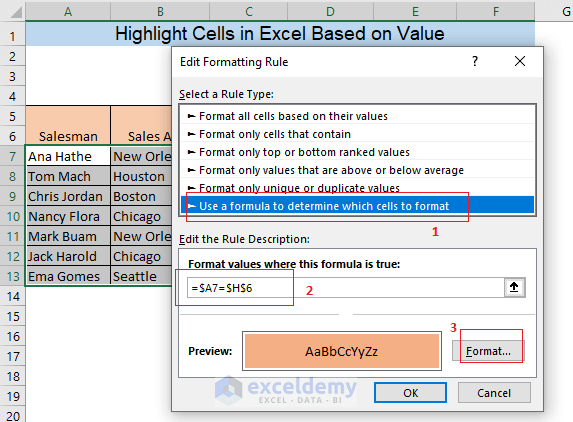
- The New Formatting Rule window will appear. Select Use a formula to determine which cells to format from Select a Rule Type.
- Type the following formula in the Format values where this formula is true box:
=$A7=$H$6Here, the formula will find the cells in your dataset where the text is the same as the drop-down selection.
- Click on Format to select the formatting style.
- Select a highlight color and other formatting options and press OK.
- Click on OK.
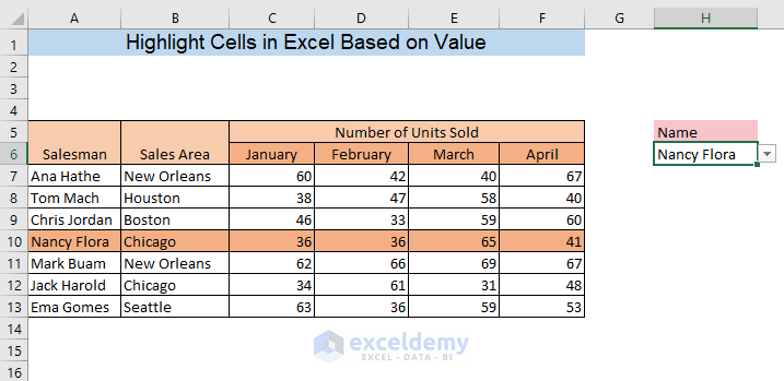
- For example, if we select Nancy Flora from the drop-down list, the sales data of Nancy Flora will be highlighted.
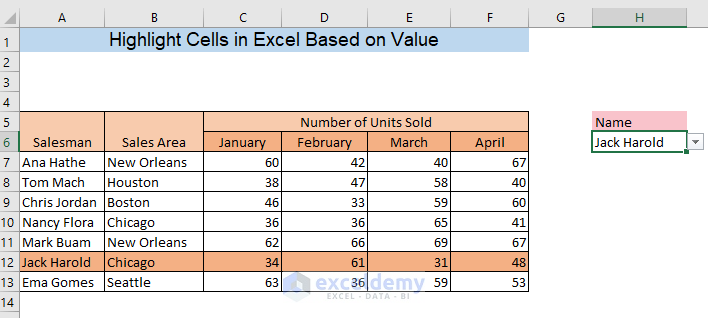
- If you change the name from the drop-down list, the highlighted cells will also be changed based on your selection.
Read More: Highlight Cells That Contain Text from a List in Excel
Download Practice Workbook
Related Articles
- How to Highlight Cell If Value Is Less Than Another Cell in Excel
- How to Highlight Cells in Excel but Not Print
- How to Highlight Cell Using the If Statement in Excel
<< Go Back to Highlight Cell | Highlight in Excel | Learn Excel
Get FREE Advanced Excel Exercises with Solutions!
