Sometimes we need to color our Excel cell to make the dataset unique, highlighted, beautiful, and easy to visualize. In this article, we will know how to color excel cells with multiple criteria, explanations, and examples.
Cell Color in Excel: Add, Change and Remove
In this article, we will demonstrate 7 effective ways to use Excel cell color. This section provides extensive details on these methods. You should learn and apply these to improve your thinking capability and Excel knowledge. We use the Microsoft Office 365 version here, but you can utilize any other version according to your preference.
1. Use Fill Color to Add Color in Cell
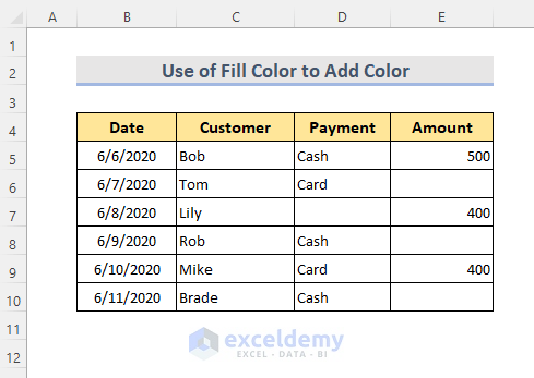
To add or change the background cell color, we can use the Fill Color option. Assuming we have a dataset (B4:E10) of customers’ payment history. Therefore, we are going to add color to the cells of the payment type.
STEPS:
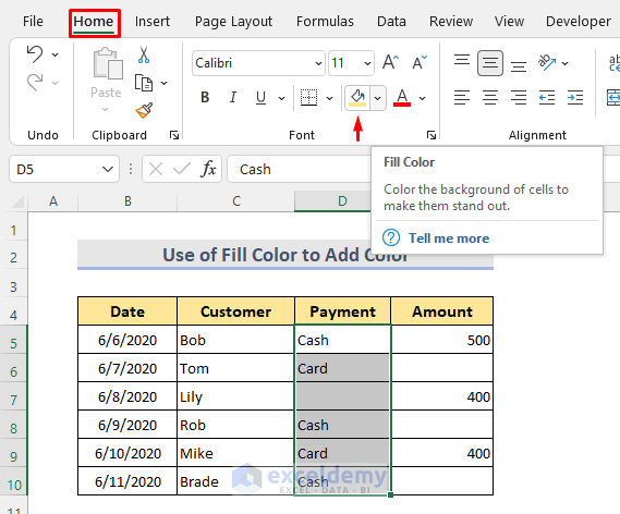
- First, select the cells (D5:D10) where we want to add color.
- Next, go to the Home tab and select the Fill color dropdown.
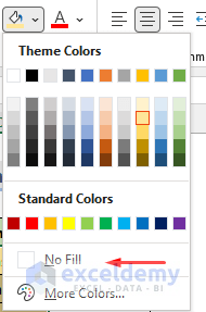
- Consequently, in the dropdown, we can see all the colors.
- Then, pick any color from the Theme Colors or Standard Colors.
- Therefore, we can also get our customized color by clicking the More Colors option.

- Afterward, selecting the dataset looks like the below.

2. Utilize Fill Color to Remove Color in Cell
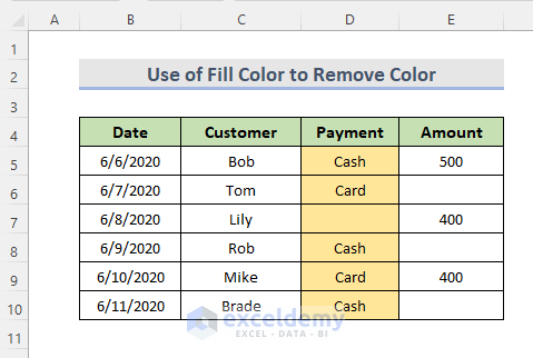
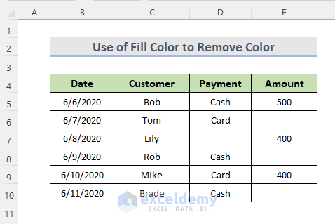
Often we need to remove the background color of a cell. Here we have a dataset of employees’ payment history and its payment type is highlighted with color. Here, we are going to remove the color of each cell.
STEPS:
- In the beginning, select the cells with color (D5:D10).
- Next, go to Home > Fill color dropdown.
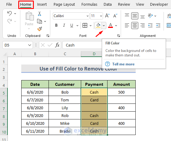
- Then, click on the No Fill option.
- Finally, the colors of the cells are removed.
3. Alternate Excel Cell Color
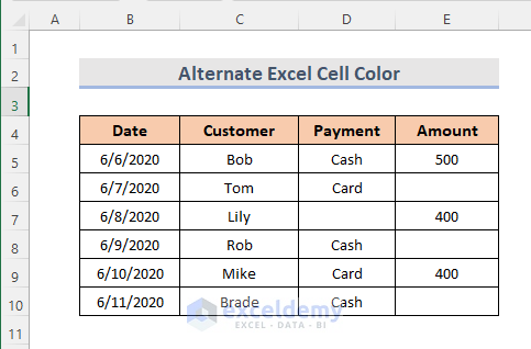
Alternating excel cell color is important to make a dataset organized. It’s very useful for analyzing a complex dataset. Let’s say we have a dataset (B4:E10). We are going to alternate the cell of the rows with the help of Color Banding & Conditional Formatting.
STEPS:
- First, select the dataset (B5:E10).
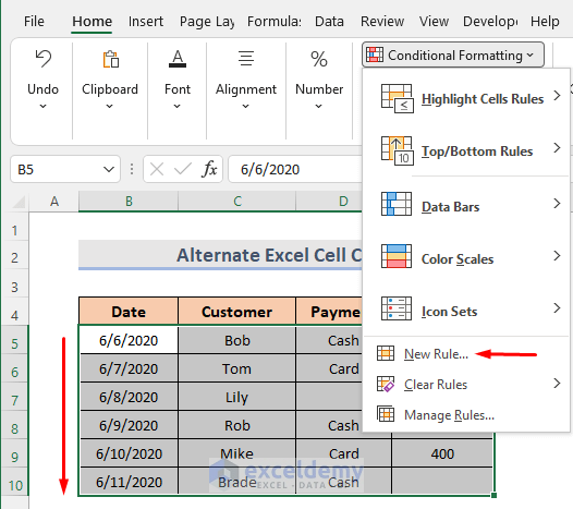
- Next, go to Home > Conditional Formatting > New Rule.
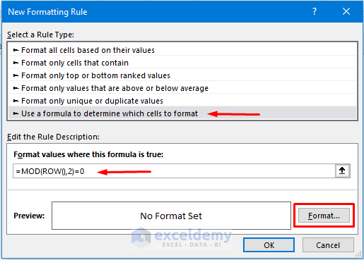
- In the New Formatting Rule window, select ‘Use a formula to determine which cells to format’.
- Consequently, in the Format values box, type the Color Banded Rows formula which will highlight every alternate row with color. The formula is:
=MOD(ROW(),2)=0- Next, click on Format.
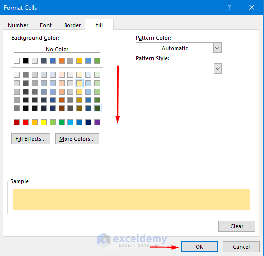
- Therefore, a Format Cells window pops up.
- Afterward, go to the Fill option and select any background color.
- Then, press OK.
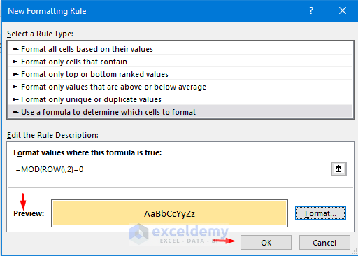
- Hence, we can see the color preview in the Preview box.
- Then, select OK.
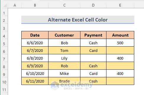
- Finally, it’s done. We can see the dataset like the below one.
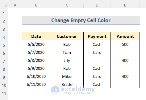
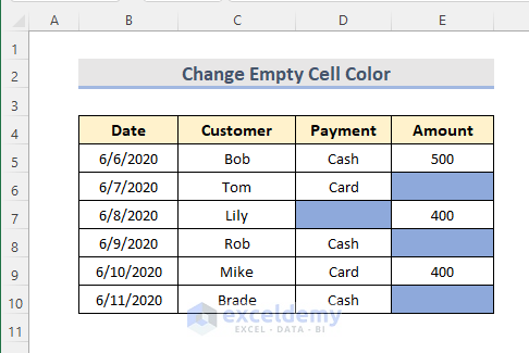
4. Change Background Color of Empty Cells in Excel
To change the background color of the empty cells dynamically, we are going to use the Conditional Formatting option. Here we have a dataset. We are going to indicate the empty cells with color.
STEPS:
- First, select the cell range B4:E10.
- After that, go to Home > Conditional Formatting > New Rule.
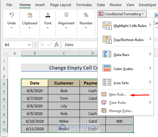
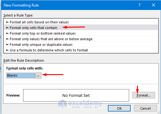
- Therefore, from the New Formatting Rule window, select the ‘Format only cells that contain’ option.
- Next, input Blank from the ‘Format only cells with’ dropdown.
- Then, click on Format.
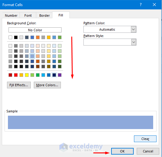
- From the Format Cells window, go to the Fill option to select the color we want.
- Now, click OK.
- Lastly, click OK to see the result.
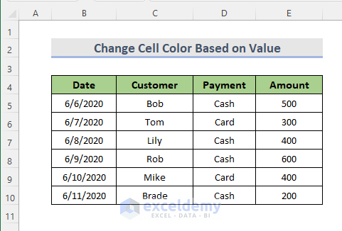
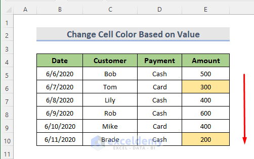
5. Dynamically Change Excel Cell’s Color Based on Value
We can dynamically change the excel cell’s background color based on a specific value. Here from the below dataset (B4:E10), we are going to indicate the values which are less than 400.
STEPS:
- First, select the range B5:E10B.
- Then, go to Home > Conditional Formatting > New Rule.
- Therefore, the New Formatting Rule window pops up.
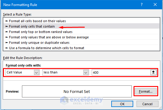
- Now, select ‘Format only cells that contain’.
- In the ‘Format only cells with’ box, we can see multiple dropdown options.
- Afterward, Select Cell Value, less than, 400 from there.
- Next, click on Format.
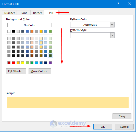
- After that, in the Format Cells window, go to the Fill section.
- Select the Background Color.
- Then, click OK.
- Again click OK.
- At last, we can see all the required cells are highlighted.
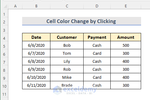
6. Apply VBA to Change Color
We can change Excel cell color by double-clicking or right-clicking on it. For that, we have input a VBA code. Assuming we have a dataset.
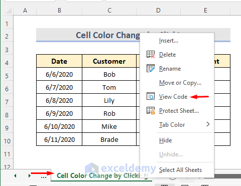
STEPS:
- First, right-click on the sheet from the sheet tab.
- Then, select View code.
- Therefore, a VBA Module window pop up.
- Now type the code:
Option Explicit
Private Sub Worksheet_BeforeDoubleClick(ByVal Target As Range, Cancel As Boolean)
Cancel = True
Target.Interior.color = vbYellow
End Sub
Private Sub Worksheet_BeforeRightClick(ByVal Target As Range, Cancel As Boolean)
Cancel = True
Target.Interior.color = vbGreen
End Sub
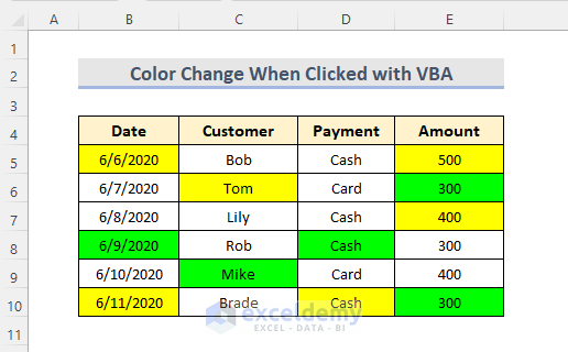
- Then, press Alt+Q and go to the worksheet.
- Lastly, right-click or double-click on it and see the result.
7. Count Cell Color
Sometimes in a big dataset, we have to count the colored cells. However, by using the Filter option with the SUBTOTAL function, we can easily sort this out. For instance, we have a dataset with colored cells. Therefore, follow the below steps to perform the task.
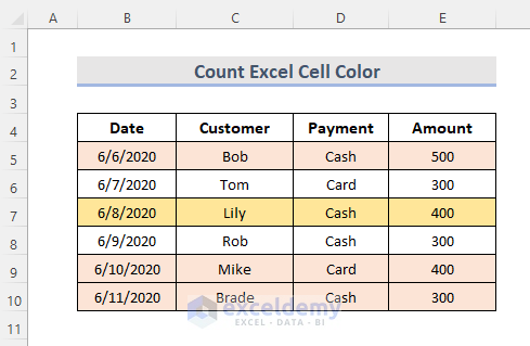
STEPS:
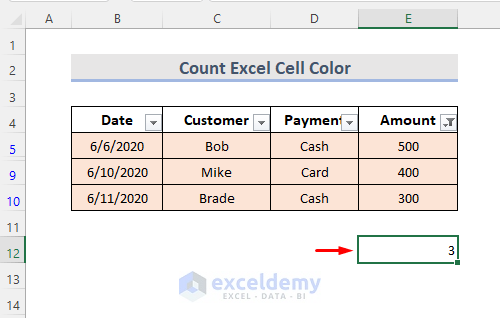
- First, select any cell (E12) below the dataset.
- Now, type the formula:
=SUBTOTAL(102,E4:E10)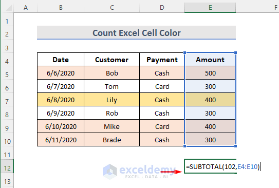
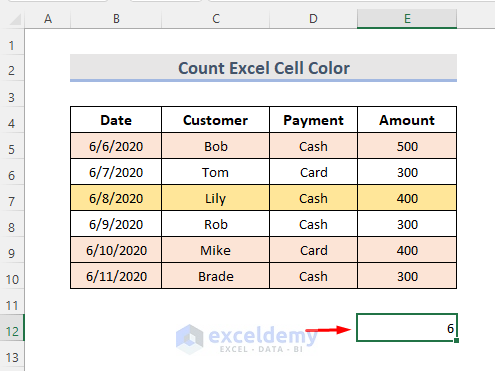
- Next, hit Enter to see the result.
- Next, select the headers of the dataset.
- Then, go to the Data tab.
- Subsequently, from Sort & Filter option, select Filter.
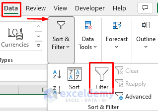
- Therefore, we can see that the filter is applied to the headers.
- After that, click on any filter dropdown of the header.
- Next, Select ‘Filter by Color’.
- Then, click on the color based on which we want to count.
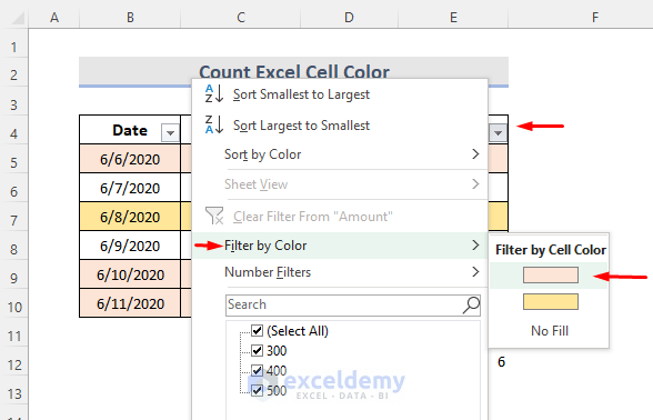
- Finally, we can see the filtered cells with their quantity in Cell E12.
Download Practice Workbook
Download the following workbook and exercise.
Conclusion
By using these methods, we can easily color cells in Excel with multiple criteria. Moreover, there is a practice workbook added. So, go ahead and give it a try. Finally, feel free to ask anything or suggest any new methods.
Color Cell in Excel: Knowledge Hub
<< Go Back to Excel Cell Format | Learn Excel
Get FREE Advanced Excel Exercises with Solutions!
