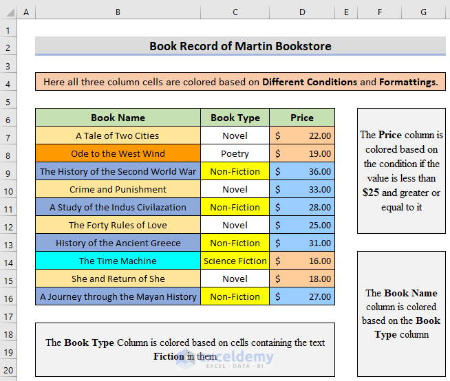
Excel Formula to Color Cell If It Has Specific Value

Here’s an overview of coloring cells based on various conditions.

Excel Formula to Color Cell If the Value Follows a Condition: 3 Approaches

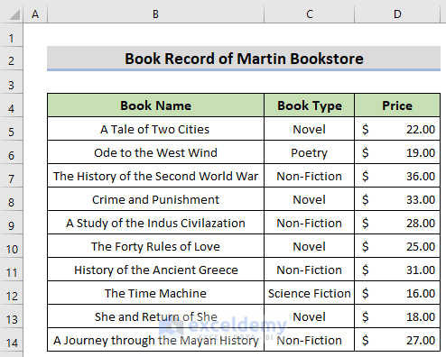
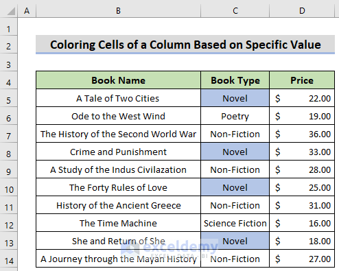
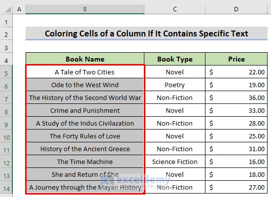
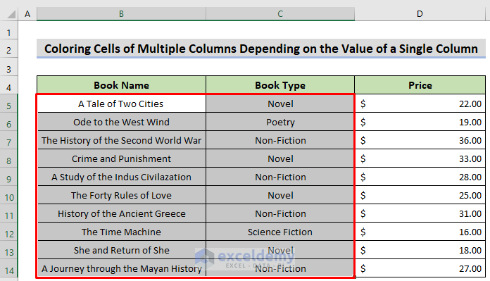
We’ve got a data set with the Names, Book Types, and Prices of some books of a book shop. We’ll color the cells based on various conditions.

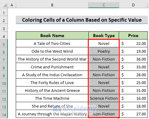
Method 1 – Excel Formula to Color Cells of a Column Based on a Specific Value

Let’s color the cells of the column Book Type if the book is a novel.

Steps:

Select the column you want to color (without the Column Header). We have selected the column Book Type (C5:C14).

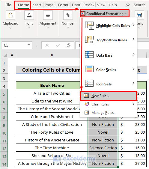
Go to the Home tab and select Conditional Formatting.
Click on New Rule.

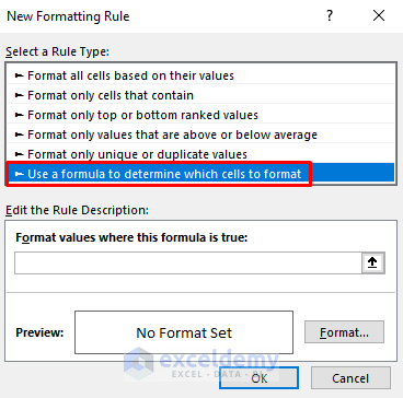
A dialog box called New Formatting Rule will open.
Click on Use a formula to determine which cells to format.

In the box called Format values where this formula is true, enter any of the following formulas:

=C5="Novel"

=$C5="Novel"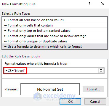

⧪ Notes

To color a single column based on some condition using Conditional Formatting, use the Relative Cell Reference or the Mixed Cell Reference (lock the column, not the row) of the first cell inside the formula.
C4 is the first cell of the column Book Type. We can use either C4 or $C4, but not C$4 or $C$4.
And the text “Novel” is my criteria. We want to find out the cells whose values are equal to the text “Novel”.

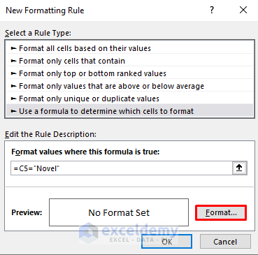
Click on Format. A dialog box called Format Cells will open.

Select your desired color from the tab Fill. We have selected light brown.

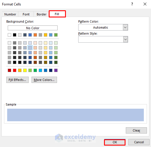
Click on OK. You will be directed back to the New Formatting Rule box.
Click on OK again.
You will find the cells of your selected column that fulfill the criteria marked in your chosen color.

⧪ Additional Example:

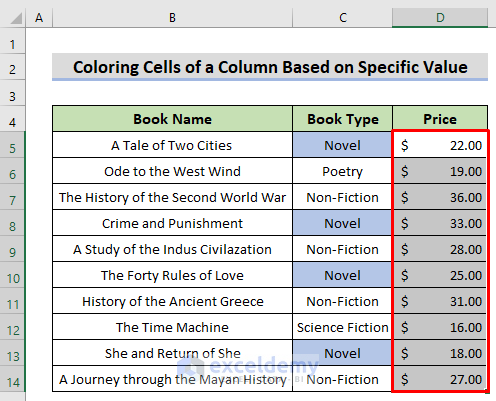
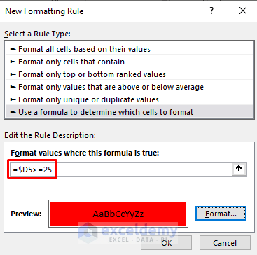
You can also color the cells of the column Price that maintain a condition in this way. Let’s color the cells that have a price greater than or equal to $25.00. The steps are all the largely the same with the following exceptions:

Select the column Price when choosing the columns.

In the New Formatting Rule box, replace the formula with this:

=D5>=25

=$D5>=25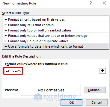

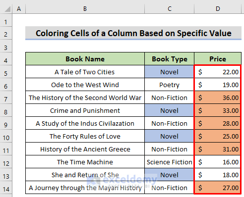
You will get the cells that contain a price greater than or equal to $25.00 marked in your chosen color.

You can use the same method to color cells of a single column that are less than a particular value. Use the less-than sign (<) in the formula.

Method 2 – Excel Formula to Color Cells of a Column If It Contains Specific Text

We’ll color the Book Names with the text “History” in them. The steps are all the same as in Method 1. The changes are:

Select the column Book Name.

For Conditional Formatting New Rule, you can use different formulas for case-sensitive matches and case-insensitive matches.

⧪ Formulas for Case-Sensitive Match:

=IF(ISERROR(FIND("History",B5)),FALSE,TRUE)

=IF(ISERROR(FIND("History",$B5)),FALSE,TRUE)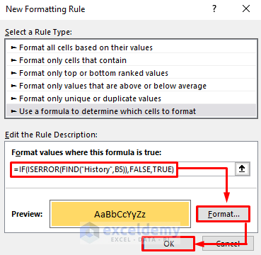

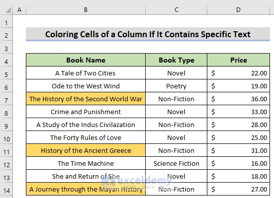
You will get the books that have the text “History” in their names marked in your desired color.

Explanation of the Formula

FIND(“History”,B4) returns an integer if it finds the text “History” (case-sensitive match) inside cell B4. Otherwise, returns a value error.
Let cell B4 doesn’t contain the text “History”. So, now the formula becomes IF(ISERROR(#VALUE!),FALSE,TRUE).
The ISERROR function returns a TRUE if it finds an error. So, now the formula becomes IF(TRUE,FALSE,TRUE).
The IF function returns the 2nd argument if the 1st argument is TRUE. Otherwise, returns the 3rd argument.
Therefore, it will return the 2nd argument, FALSE.
Similarly, if cell B4 had contained the text “History”, the formula would have returned TRUE.

Note

This formula works for a case-sensitive match. So “history” or “HISTORY” in place of “History” won’t work.

⧪ Formulas for Case-Insensitive Match:

=IF(ISERROR(SEARCH("history",B4)),FALSE,TRUE)

=IF(ISERROR(SEARCH("history",$B4)),FALSE,TRUE)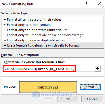

You will get the books that have the text “History” or “history” or “HISTORY” or so on in their names marked in your desired color.

Explanation of the Formula

SEARCH(“history”,B4) returns an integer if it finds the text “history” (case-insensitive match) inside cell B4. Otherwise, returns a value error.
Let the cell B4 doesn’t contain the text “history”. So, now the formula becomes IF(ISERROR(#VALUE!),FALSE,TRUE).
The ISERROR function returns a TRUE if it finds an error. So, now the formula becomes IF(TRUE,FALSE,TRUE).
The IF function returns the 2nd argument if the 1st argument is TRUE. Otherwise, returns the 3rd argument.
Therefore, it will return the 2nd argument, FALSE.
Similarly, if cell B4 had contained the text “history”, the formula would have returned TRUE.

Note

This formula works for a case-insensitive match. So “History” or “HISTORY” in place of “history” will also work.

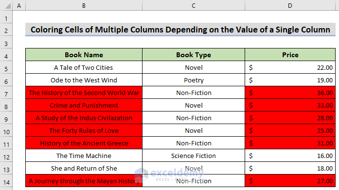
Method 3 – Excel Formula to Color Cells in Multiple Columns Depending on the Value of a Single Column

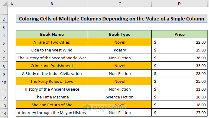
We’ll color the columns Book Name and Book Type depending on the values of the column Book Type. We’ll color a book only if it’s a Novel. The steps are the same as in Method 1, with the following exceptions:

Select both of the columns when applying Conditional Formatting.

Use the following formula with the Mixed Cell Reference in the formula box for the New Formatting Rule dialog.

=$C5="Novel"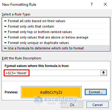

Choose your desired color from the Format Cells dialogue box.
Click OK twice. You will get the cells in both the columns marked in your chosen color if the book is a novel.

⧪ Additional Example:

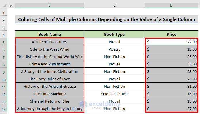
You can also color the cells of the column Book Name and Price if the price is greater than or equal to $25.00 in this way:

Select the two columns Book Name and Price.
Open Conditional Formatting and New Rule.

Enter this formula with a Mixed Cell Reference:

=$D5>=25

Choose your desired color from the Format Cells dialogue box.
Click OK twice. You will get the cells in both the columns marked in your chosen color if the price is greater than or equal to $25.00.

Things to Remember

To color the cells of a single column, you can use either the Relative Cell Reference or the Mixed Cell Reference (Locking the Column) in the formula.
To color the cells of multiple columns based on a single column, you must use the Mixed Cell Reference (Locking the Column) in the formula.
The FIND function goes for a case-sensitive match, and the SEARCH function goes for a case-insensitive match.

Frequently Asked Question

Why must we use Mixed Cell Reference while coloring cells of multiple columns based on a single column?

When we select multiple cells and apply a formula to them through Conditional Formatting, the formula is applied to the first cell of the selected range.

Then, it’s copied to the rest of the selected cells, just like we copy a formula in our worksheet from one cell to another by dragging the Fill Handle.

Let’s understand it through an example.

When we apply the formula =C4=”Novel” to the selected range B4:C13 through Conditional Formatting, cell B4 gets the formula =C4=”Novel”.

Then cell B5 gets =C5=”Novel”.

Cell B6 gets =C6=”Novel”.

This is OK. For column B, there will be no problem.

But when we go to column C, cell C4 will get the formula =D4=”Novel”. Because the formula will be copied rightwards.

This is not what we want. We want to color cell C4 based on the value of cell C4, that whether it contains “Novel” or not.

So, we want the formula =C4=”Novel” in cell C4, not =D4=”Novel”.

That’s why we need to insert the Mixed Cell Reference. If we use =$C4=”Novel”, it will remain =C4=”Novel” when it is copied from column B to column C.

But we lock only the column, not the row, because we want the cell reference to increase by 1 when it is copied downwards.

Download the Practice Workbook

Formula to Color a Cell If the Value Follows a Condition.xlsx

<< Go Back to Color Cell in Excel | Excel Cell Format | Learn Excel

Get FREE Advanced Excel Exercises with Solutions!