To learn about the CELL COLOR A1 you need to understand the CELL function first. This function returns information about the cell. The syntax of the CELL function is:
CELL(info_type, [reference])| Argument | Required/Optional | Explanation |
|---|---|---|
| info_type | Required | A text value out of 12 different values that specify what type of cell info you want. |
| reference | Optional | A particular cell that you want the info about. If [reference] is provided, the function will return info_type of the then selected cell or active cell in case of a range. |
There are 12 types of information about a particular cell. And cell “Color” is one of them. The info_type has to be entered with a double quotation (“ “) marks in the CELL function.
“color”: Returns 1 if the cell is formatted in color for Negative values,
or returns 0 (zero) otherwise.
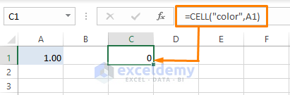
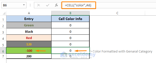
While using the “color” type you can use the cell reference, which can be A1. So, the formula will look something like:
=CELL("color",A1)And while using the formula in Excel without color formatting and a negative value in cell A1, the output will be similar as shown in the following screenshot.
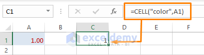
On the other hand, if the value gets color formatted with negative numbers, the formula returns 1 as shown in the following image.
For the purpose of this tutorial, we’ll discuss and demonstrate only examples regarding the color info_type.
Example 1 – Fetching Cell Color Info
The CELL function provides information about a cell, and one of its info_type arguments is Color.
To check if a cell is color-formatted for negative values, use the formula =CELL(“color”,[reference]).
This formula returns 1 if the [reference] cell is color formatted for negative value otherwise 0.
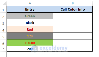
For instance, if we have color-formatted entries in cells, and we want to check which ones are color formatted for negative values, follow these steps:
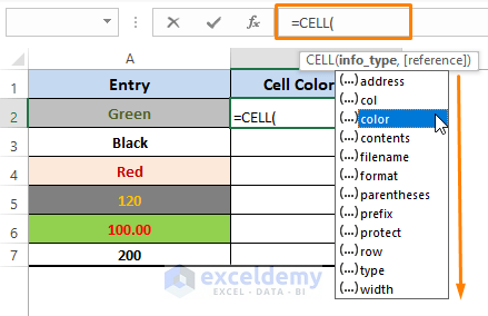
- Write =CELL( in the Formula Bar. Multiple (12 to be exact) info_type arguments appear.
- Select Color.
- Enter the [reference] (i.e., A2, we could use A1 if we didn’t use a table header) following a comma (,) as shown in the below formula.
=CELL("color",A2)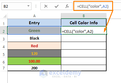
- Press ENTER.
- If A2 is color-formatted for a negative value, the formula will return 1; otherwise, it returns 0.
- Drag the Fill Handle down.
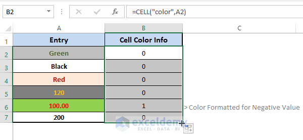
Only cell A6 is color formatted for a negative value, as a 1 is returned.
Test this formula for any color-formatted negative values, and it consistently returns 1.
Example 2 – Showing Pre-set Text Depending on Values
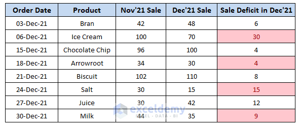
Suppose we have a dataset with Product Sales for Nov’21 and Dec’21, and we calculate the Sale Deficit for Dec’21 relative to Nov’21.
We color-formatted deficit values that are less than Nov’21 sales using Conditional Formatting.
- To display “Positive” or “Negative” text for each cell based on color formatting, use the formula in H5:
=IF(CELL("color",F5),"Negative","Positive")-
- Here, F5 represents the cell containing the deficit value.
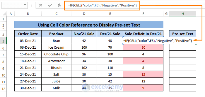
- Press ENTER then Drag the Fill Handle down to populate the results in the remaining cells.
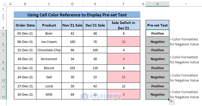
The formula returns Negative for cells with color-formatted negative values.
Example 3 – Direct Used in Formula
We will directly use the “color” argument from the CELL function in a formula to display text strings based on certain conditions.
Suppose we have a dataset, and we want to display either YES or NO depending on the quantity (Negative Deficit) of a specific product.
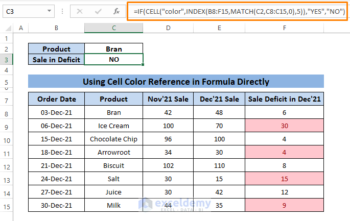
- Paste the following formula in any blank cell (i.e., C3).
=IF(CELL("color",INDEX(B8:F15,MATCH(C2,C8:C15,0),5)),"YES","NO")Inside the formula:
- The MATCH function matches the cell reference C2 to the range C8:C15 and returns the value as row_num.
- The INDEX function then matches the row_num and col_num (i.e., we input 5).
- The CELL function identifies whether the particular cell has a color-formatted negative value or not.
- The IF function displays YES or NO based on whether the cell is color-formatted or not.
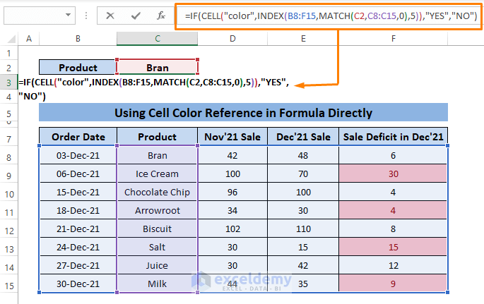
- After pressing ENTER, you’ll see the YES or NO string depending on the color-formatted negative value, as shown in the screenshot.
We color-formatted values whenever the difference between two months’ sales (Dec’21-Nov’21) results in a negative value.
Color Formatting Considerations
- If you apply formatting with any color for negative values and then use the =CELL(“color”,[reference]) formula, it may not show 1 as expected.
- To address this issue:
- Click on the icon (shown in the screenshot) in the Home Tab Font section.
- The Format Cells window appears. Select Number (in the Category option).
- Choose the 2nd option under Negative numbers (as shown in the screenshot).
- Click OK.
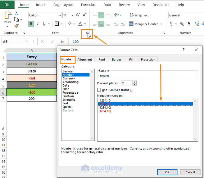
When you apply the formula again, it will correctly return 1 for color-formatted negative values.
Remember to color format the negative values to ensure the formula behaves as expected.
Download Excel Workbook
You can download the practice workbook from here:
Related Articles
- How to Color Code Cells in Excel
- Excel Formula to Change Cell Color Based on Text
- How to Change Cell Color Based on a Value in Excel
- How to Fill Color in Cell Using Formula in Excel
- How to Fill Cell with Color Based on Percentage in Excel
- Excel Formula to Color Cell If It Has Specific Value
- How to Change Text Color with Formula in Excel
- How to Apply Formula Based on Cell Color in Excel
- VBA to Change Cell Color Based on Value in Excel
<< Go Back to Color Cell in Excel | Excel Cell Format | Learn Excel
Get FREE Advanced Excel Exercises with Solutions!
