How to Change Cell Color Based on a Value in Excel (5 Ways)

Method 1 – Dynamically Change Cell Color Based on a Value

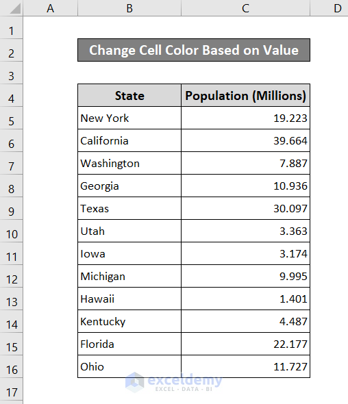
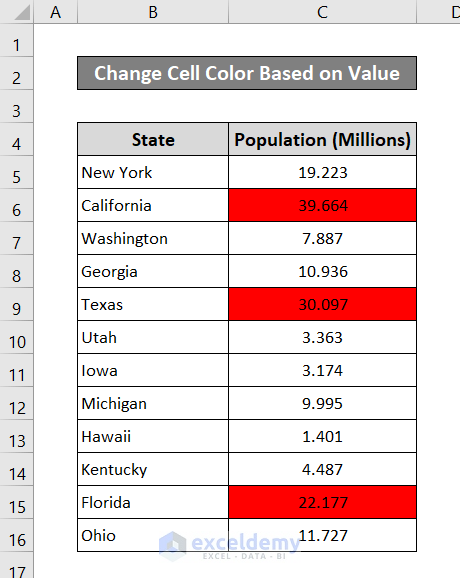
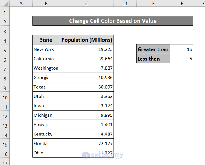
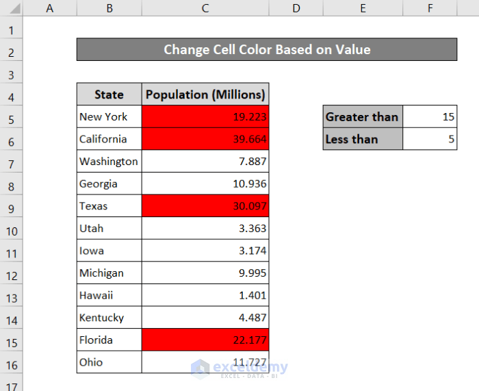
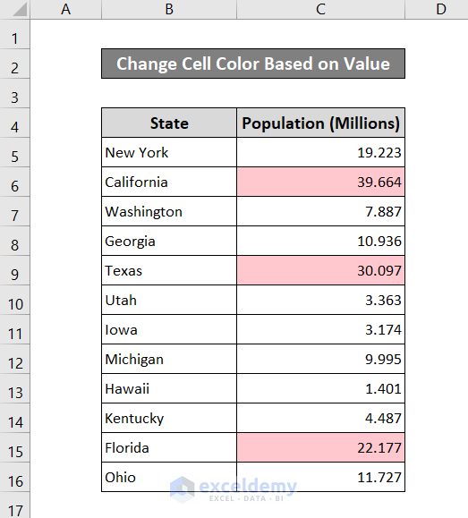
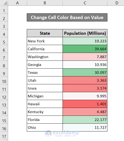
Consider the following dataset that shows U.S. state populations. We’ll divide the population numbers into 3 categories: above 20 million, below 5 million, and in between.

Steps:

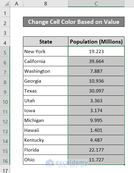
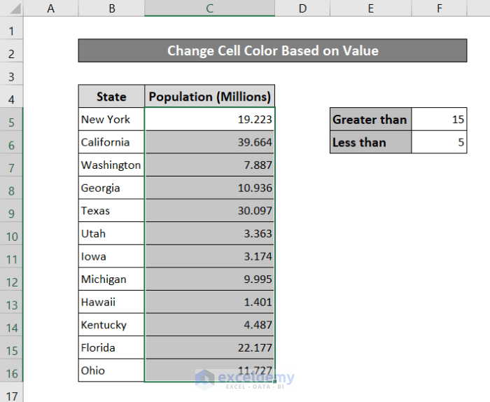
• Select the range of cells you want to format.

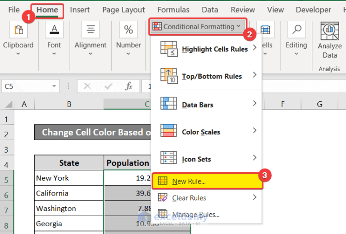
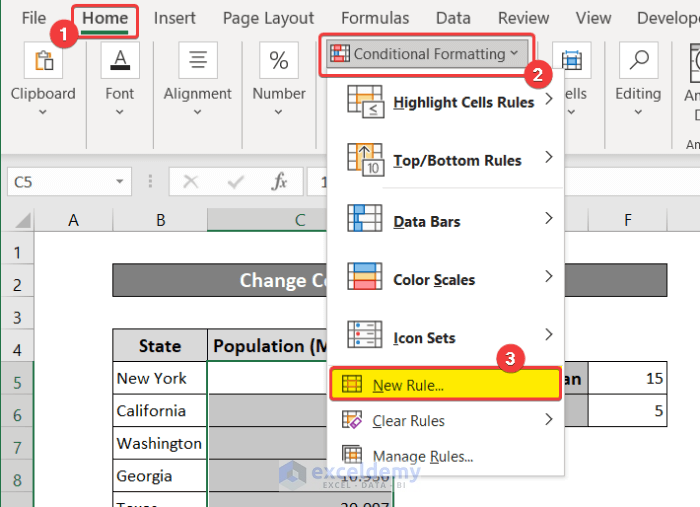
• Select Conditional Formatting under Home.
• Select New Rule from the drop-down list.

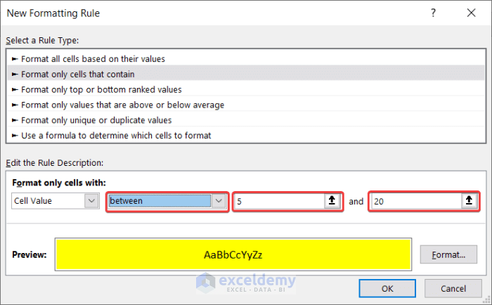
• In the New Formatting Rule box, select Format only cells that contain under Select a Rule Type.
• In the Rule Description, choose the condition greater than or equal to and put in the value 20.

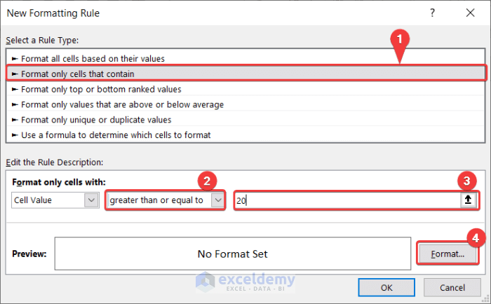
• Click on Format.
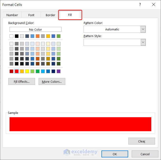
• Go to the Fill tab in the Format Cells box and pick a background color. We chose red for the example.

• Click on OK on both Format Cells and New Formatting Rule.

• Repeat the process and put between as condition and 5 and 20 as values.

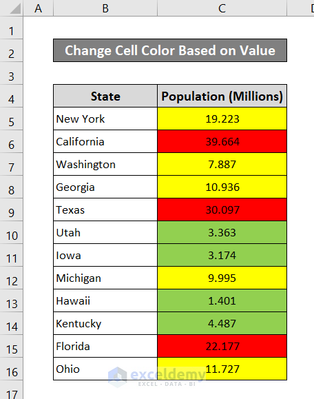
• Repeat for lower than or equal to 5 and you will have your cell color changed according to the values for the full range.

Method 2 – Change Cell Color Based on a Value of Another Cell

We have selected two values in cells F5 and F6 as a source to customize from.

Steps:

• Select the range of cells you want to format.

• Select Conditional Formatting and choose New Rule.

• In the New Formatting Rule box, select Format only cells that contain under Select a Rule Type.
• In Rule Description, choose the condition to be greater than and put the following formula:

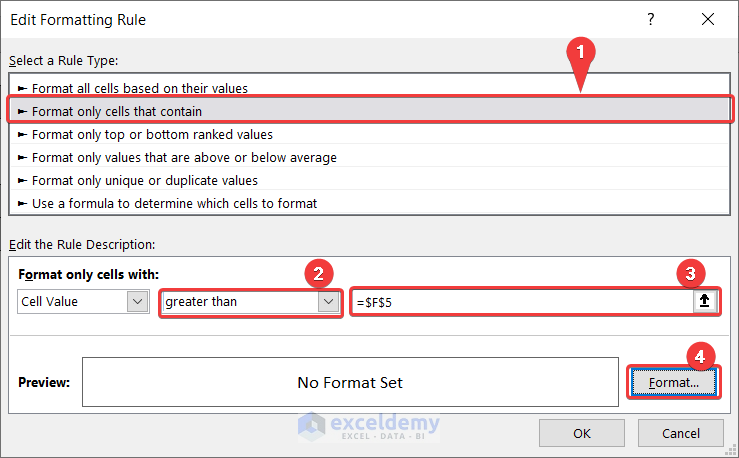
• Click on Format.
• In the Fill tab, select a background color.

• Click on OK on both Format Cells and the New Formatting Rule.

• Repeat the same procedure for changing color by selecting less than as the condition and referencing cell F6: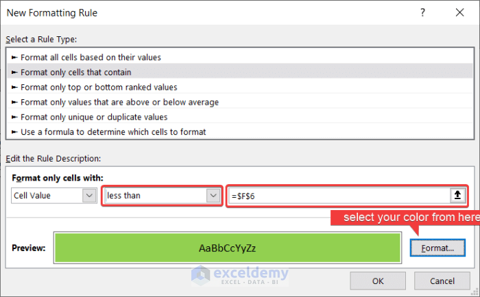

• Here’s the result.

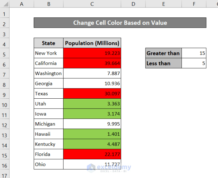
• If the values in cells F5 or F6 change, the colors from the range of cells C5:C16 will change accordingly.

Read More: VBA to Change Cell Color Based on Value in Excel

Method 3 – Using the Quick Formatting Option to Change Cell Color in Excel

Steps:

• Select the cell and hover over the bottom-right corner of the selected range. A Quick Analysis Toolbar Icon will appear.

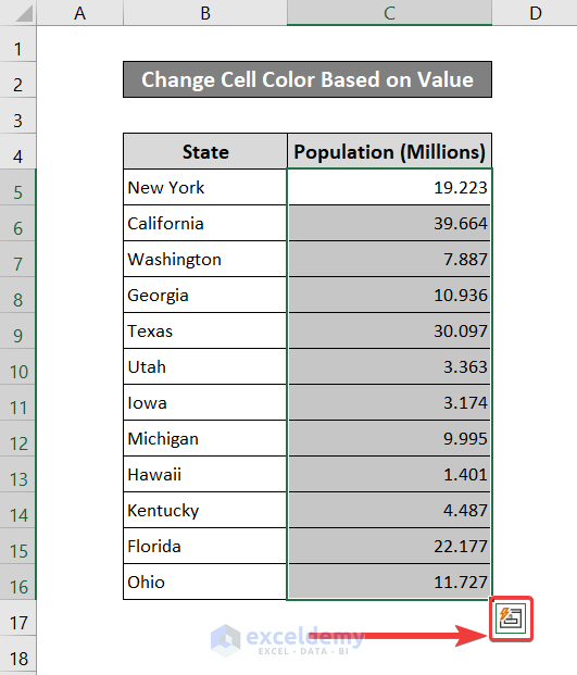
• Click on it.
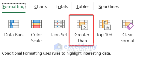
• In the Formatting tab, select Greater Than.

• In the Greater Than tab, select the value above which the cells within the range will change color. We have put 20.

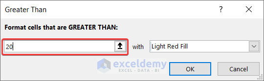
• You can also change the color.
• Click OK.

You can also select the Color Scale option in the Formatting tab from the Quick Access Toolbar Icon to have a different range of colors for the column.

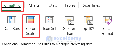
You will have a wide range of color cells based on the percentiles: red for the lowest, to white, to green for the highest.

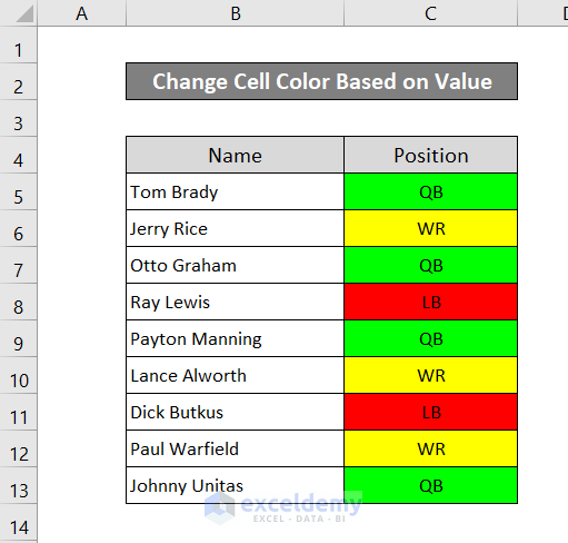
Method 4 – Change Cell Color Permanently Based on a Value

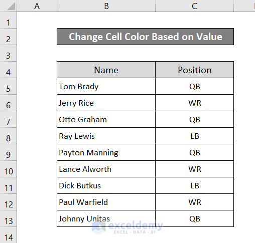
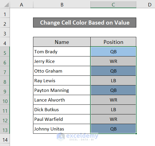
We have three values as positions and will show you how to have three different colors for QB, LB, and WR.

Steps:

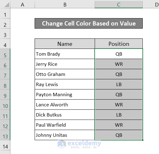
• Select the range of cells you want to modify.

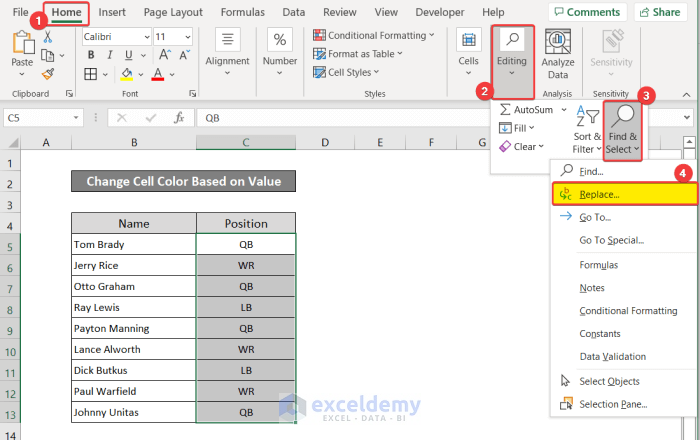
• In the Home tab, select Find & Select from the Editing section.
• From the drop-down list, select Replace.

• In the Find and Replace box, put QB in the Find what box.
• Put QB in the Replace with box and change the format to the right.

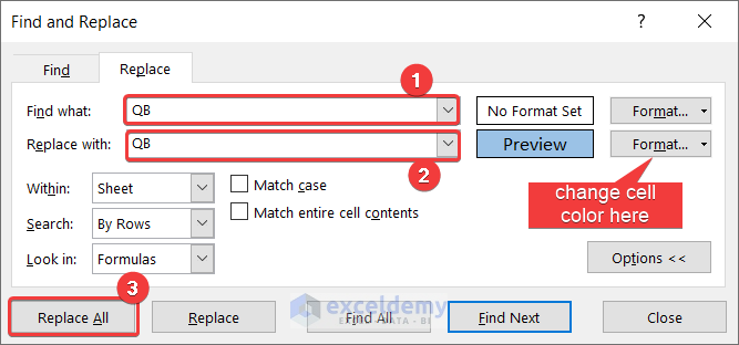
• Select Replace All and you will have all the boxes with QB as the value will change to this color.

• You can keep changing colors for cells with different values by replacing the text and formatting, then pressing Replace All.
• After changing colors for all three values, close the box.

Method 5 – Change Cell Color Based on a Value Using Excel VBA

You may need to enable the Developer tab if you don’t see it on your ribbon.

Steps:

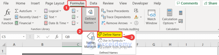
• Select your cells and go to the Formulas tab.
• Select Define Name under the Defined Names group.

• Name your range in the Edit Name. We will be using “Positions”. Name it the same if you want to copy the VBA code.

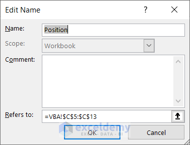
• Click on OK.
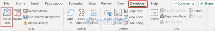
• Go to the Developer tab and select Visual Basic.

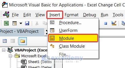
• In the VBA window, select Insert and choose Module.

• Insert the following code into the module:

Sub Change_Cell_Color()
Dim cell_value As Range
Dim stat_value As String
Dim rng As Range
Set rng = Range("Position")
For Each cell_value In rng
stat_value = cell_value.Value
Select Case stat_value
    Case "QB"
    cell_value.Interior.Color = RGB(0, 255, 0)
    Case "WR"
    cell_value.Interior.Color = RGB(255, 255, 0)
    Case "LB"
    cell_value.Interior.Color = RGB(255, 0, 0)
End Select
Next cell_value
End Sub

• Save your code.
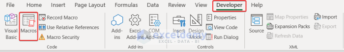
• Go to Macros under the Developers tab.

• In the Macro box, select the code you have just created and run.

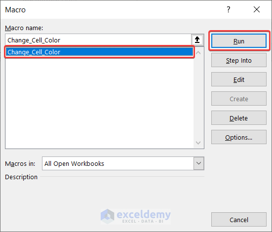
• Your cell colors will change depending on the value.

Download the Practice Workbook

Related Articles

• How to Color Code Cells in Excel
• Excel Formula to Change Cell Color Based on Text
• How to Fill Color in Cell Using Formula in Excel
• How to Fill Cell with Color Based on Percentage in Excel
• Excel Formula to Color Cell If It Has Specific Value
• How to Change Text Color with Formula in Excel
• How to Apply Formula Based on Cell Color in Excel

<< Go Back to Color Cell in Excel | Excel Cell Format | Learn Excel