How to Apply Formula Based on Cell Color in Excel (5 Easy Ways)

Here’s an overview of applying formulas in cells based on the colors they have.

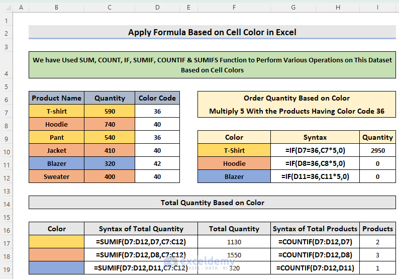
Apply Formula Based on Cell Color in Excel: 5 Examples

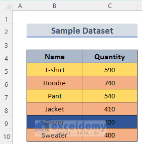
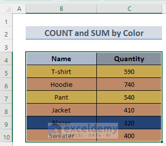
We will use the following colorful dataset to explain the methods. The dataset has two columns for Name and Quantity. There are 3 different colors in the rows, which we’ll use as criteria.

Example 1 – Excel SUBTOTAL Formula with Cell Color

Steps:

In Cell C6, insert the following formula to get the Count of products in the list:

=SUBTOTAL(102,C5:C10)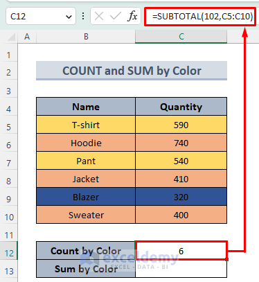

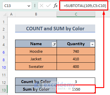
To get the Sum of the quantities of the product, use the following formula in Cell C14:

=SUBTOTAL(109,C5:C10)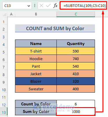

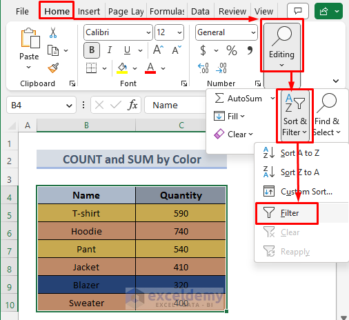
Select the whole dataset.

From the Home tab, select Filter in the Sort & Filter drop-down menu.

You will find two arrows in the columns of the dataset.

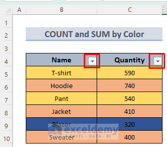
Click on the arrow symbol of the column Name.
Choose Filter by Color.
Choose the color that you want to filter.

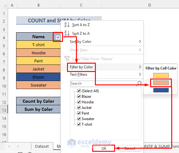
Click OK.
The values in Count by Color and Sum by Color will change.

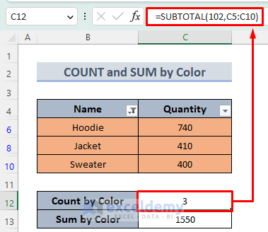
The results show the count and sum of only the filtered data.

How Does the Formula Work?

SUBTOTAL takes two arguments function_name and ref1. In the function_name it takes 102 to count the number of data and 109 to return the sum of the quantities. Specifically, 102 and 109 don’t count the cells (unlike functions 2 and 9, which do).
As a reference, both formulas take a range.
When the filter is applied, some rows are hidden, so the formulas won’t account for them.

Example 2 – Excel COUNTIF and SUMIF Formula by Cell Color

Case 2.1 – COUNTIF Formula with Cell Color

Steps:

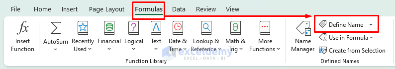
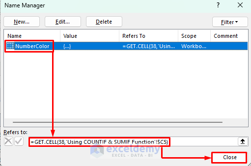
From the Formulas tab, select Define Name.

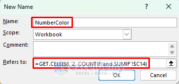
A box will appear. Write a name (in this case we wrote NumberColor in the Name: section).
In Refers to, use the following formula:

=GET.CELL(38,'2. COUNTIF and SUMIF'!$C14)

Click OK.

The name will show in the Name Manager box.
Click Close.

Make a new column D for Color Code.
In Cell D5, apply the formula:

=NumberColor

Press Enter and drag the formula using the Fill handle icon to the rest of the column.

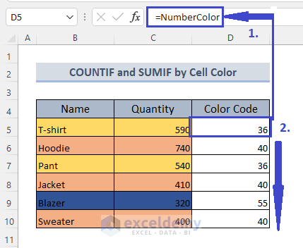
You will get the code for all the colors present in the dataset.
In G5, insert this formula:

=COUNTIF(D5:D10,$D$5)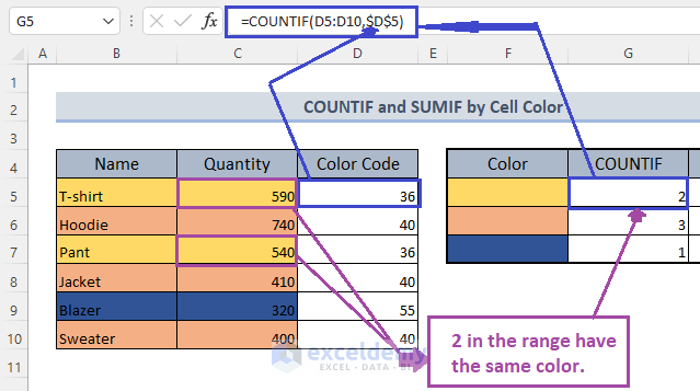

In Cell G6, insert the following:

=COUNTIF(D5:D10,$D$6)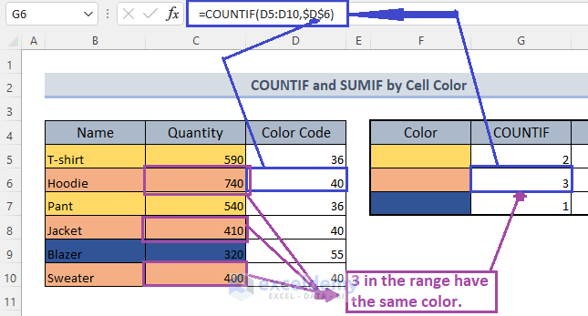

In Cell G7, insert the following.

=COUNTIF(D5:D10,$D$9)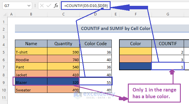

For more accurate results, you should fetch the possible colors from an independent table (such as in column F) and use those values instead.

Case 2.2 – SUMIF Formula with Cell Color

Steps:

Use the following formula in Cell H5:

=SUMIF(D5:D10,$D$5,C5:C10)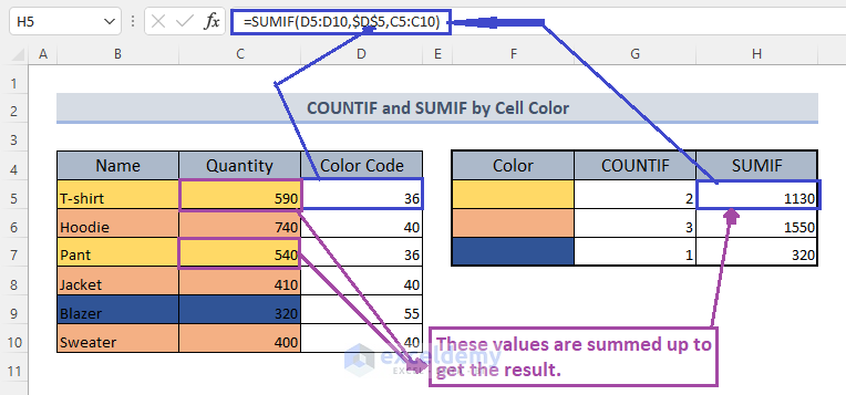

Insert the following in Cell H6,

=SUMIF(D5:D10,$D$6,C5:C10)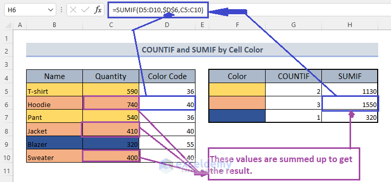

Insert the following formula in Cell H7:

=SUMIF(D5:D10,$D$9,C5:C10)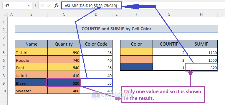

How Does the Process with Formulas Work?

The formula using the GET.CELL function takes 38 to return code color and cell reference of which the code it will return.
Using the Color codes, we have applied the COUNTIF and the SUMIF formula to get the count and sum of the data range with color code criteria.

Example 3 – Excel IF Formula by Cell Color

We have the same price per piece for products like hoodies, jackets, and sweaters. We want to calculate the total price for the total quantities of these products.

Steps:

We have created the NumberColor property using the Define Name and used it to find color codes (See Example 2).
Insert this formula in Cell E5:

=IF(NumberColor=40,C5*$C$13,0)

Press Enter.
Drag the Fill handle icon to get the result for the rest of the data.

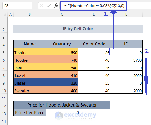
The result showed values only for the products with the same color having color code 40 while zero (0) for the rest.

How Does the Formula Work?

The IF formula takes NumberColor to be equal to 40.
If the logic is true, it will multiply the quantity with the price per piece (5). Otherwise, it will show 0.

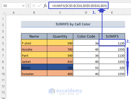
Example 4 – Excel SUMIFS Formula by Cell Color

Steps:

In Cell E5 insert the formula:

=SUMIFS($C$5:$C$10,$D$5:$D$10,$D5)

Press Enter.
Use the Fill handle icon to drag the result for the rest of the cases.

How Does the Formula Work?

The SUMIFS formula takes the sum_range C5:C10 as absolute references for quantities. Followingly, it takes the color code range which is also in absolute reference form.
The criteria are set for the first cell of the color code column which is D5. In this case, only the column is in absolute reference form while the rows are in relative reference form. It is because it will drag the Fill handle icon for the rest of the column by changing the row numbers as required.

Example 5 – Excel VBA Macro to Use Excel Formula by Cell Color

The first sub-method will find the color code and then apply them to apply the COUNTIF and the SUMIF formulas.

Note: VBA Macro cannot recognize similar colors and so we modified our dataset with different colors.

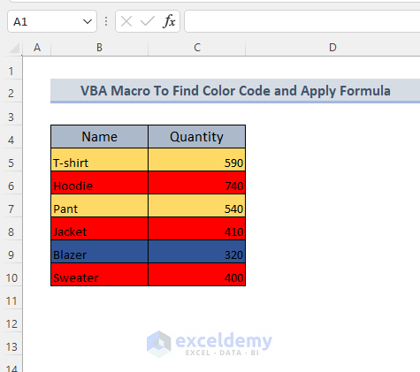
Case 5.1 – VBA Macro to Find the Color Code

Steps:

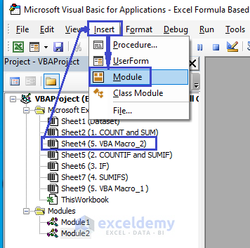
Press Alt + F11.
This will open up the VBA Macro window. Select your sheet.
From the Insert tab, click on Module.

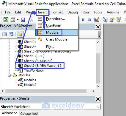
The General window will open.

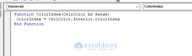
Copy and paste the following code in the General window.

Code:

Function ColorIndex(CellColor As Range)
ColorIndex = CellColor.Interior.ColorIndex
End Function

Save the file as an Excel Macro-Enabled Workbook (.xlsm).
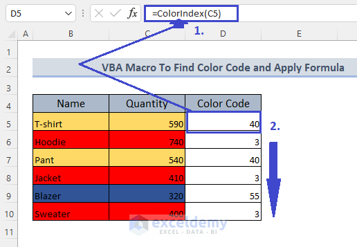
Open your sheet and insert the following formula in Cell D5:

=ColorIndex(C5)

Press Enter and drag the Fill handle to get the result for the rest of the data.

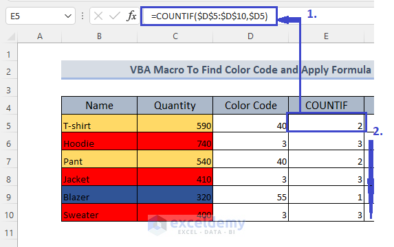
In Cell E5, insert the formula below:

=COUNTIF($D$5:$D$10,$D5)

Press Enter and drag the formula down.

Use the formula given below in Cell F5:

=SUMIF($D$5:$D$10,$D5,$C$5:$C$10)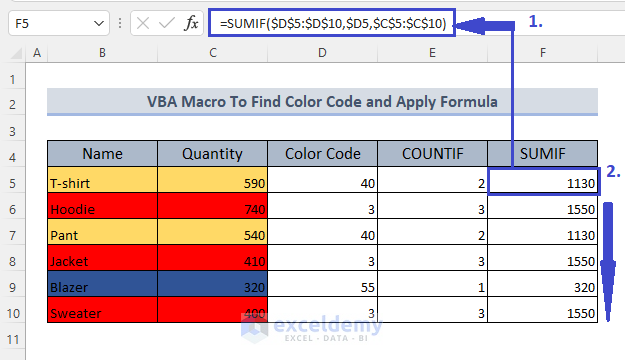

For this case, you have to find out the sum using color code. However, you can directly do the sum by writing a code. This will be explained in the next sub-method.

How Does the Process with Formulas Work?

We have created ColorIndex using the code and keeping the argument as the range of the data. Using this we get the color codes.
Next, we used the COUNTIF formula to get the count result for that particular color code.
Lastly, we used the SUMIF formula to get the sum based on the color code.

Case 5.2 – VBA Macro to Sum

Steps:

Press Alt + F11 to open the VBA Macro Window.
Select your sheet and insert a Module from the Insert tab.

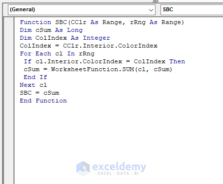
The General window will open. Copy and paste the following code in the General window.

Code:

Function SBC(CClr As Range, rRng As Range)
Dim cSum As Long
Dim ColIndex As Integer
ColIndex = CClr.Interior.ColorIndex
For Each cl In rRng
If cl.Interior.ColorIndex = ColIndex Then
cSum = WorksheetFunction.SUM(cl, cSum)
End If
Next cl
SBC = cSum
End Function

Open your worksheet.
In Cell D5, insert the following formula:

=SBC($C5,$C$5:$C$10)

Press Enter and drag the result using the Fill handle to the end of the data range.

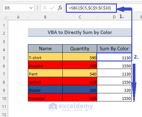
You will get the result as shown in the above picture.

How Does the Process with Formulas Work?

We created a formula with the name SBC through the code we have written in the General window for this worksheet.
After that, we used the formula with a range of data and criteria as the particular cell of quantities.

Things to Remember

Use different colors in case of applying VBA Macro.
Save the Excel file with the .xlsm suffix in case the file has VBA Macro codes within it.

Download the Practice Workbook

Formula Based on Cell Color.xlsm

<< Go Back to Color Cell in Excel | Excel Cell Format | Learn Excel

Get FREE Advanced Excel Exercises with Solutions!

4 Comments

Emil Lazar Jan 25, 2023 at 10:05 PM

That’s a very nice article, just what I was looking for (count cells of a certain color) and more.
- Reply
  Shamima Jan 26, 2023 at 9:12 AM
  
  Hello, Emil Lazar!
  
  Thanks for your appreciation. Stay in touch with ExcelDemy to get more useful articles.
  
  Regards
  ExcelDemy
Sia Jun 21, 2024 at 1:51 AM

Using this code, for cells where the quantity is less than one in each cell, I get a sum result = 0, even though the sum of the individual cells can be less than one, equal to 1, or greater than one.
Example
Cell A1 = .20
Cell B1 = .20
Cell C1 = .20
The sum of these cells is .60. The result after rounding up to the nearest integer would be 1.

How can I alter the code to show the the sum result to rounded up to the nearest integer?
- Reply
  Shamima Sultana Jun 23, 2024 at 9:55 AM
  Hello Sia,
  
  To modify the VBA code to round up the sum result to the nearest integer, you can use the Application.WorksheetFunction.Ceiling function. Use the following updated code to get your desired result:
```
Function SumByColor(CellColor As Range, SumRange As Range)
    Dim SumResult As Double
    Dim Cell As Range

    Application.Volatile

    For Each Cell In SumRange
        If Cell.Interior.Color = CellColor.Interior.Color Then
            SumResult = SumResult + Cell.Value
        End If
    Next Cell

    SumByColor = Application.WorksheetFunction.Ceiling(SumResult, 1)
End Function
```
  The formula will be : =SumByColor(A1, A1:C1)
  
  Regards
  ExcelDemy

How to Apply Formula Based on Cell Color in Excel (5 Easy Ways)

Apply Formula Based on Cell Color in Excel: 5 Examples

Example 1 – Excel SUBTOTAL Formula with Cell Color

Example 2 – Excel COUNTIF and SUMIF Formula by Cell Color

Case 2.1 – COUNTIF Formula with Cell Color

Case 2.2 – SUMIF Formula with Cell Color

Example 3 – Excel IF Formula by Cell Color

Example 4 – Excel SUMIFS Formula by Cell Color

Example 5 – Excel VBA Macro to Use Excel Formula by Cell Color

Case 5.1 – VBA Macro to Find the Color Code

Case 5.2 – VBA Macro to Sum

Things to Remember

Related Articles

Leave a reply Cancel reply