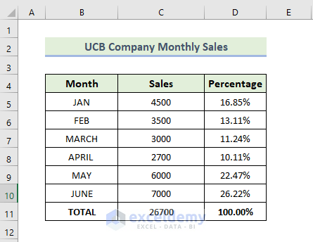
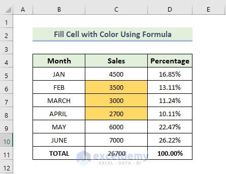
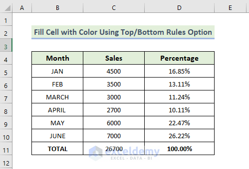
How to Fill Cell with Color Based on Percentage in Excel (6 Methods)

Here’s a dataset that contains the percentage of a company’s sales from different months. We’ll fill those cells with colors depending on the percentage.

Method 1 – Using a Formula to Fill Cell with Color Based on Percentage

We’ll use a single color to fill all cells that contain values between 10 and 15 percent.

Steps:

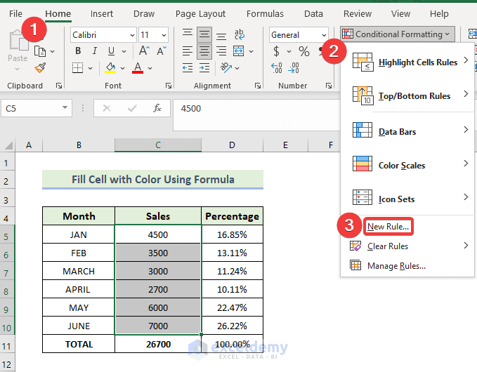
Select the range of cells C5:C10.
Go to the Home tab, select Conditional Formatting, and choose New Rule.

When the New formatting Rule dialog box appears, select the option Use a formula to define which cells to format.
In the Format values where this formula is true box, insert the following formula:

=AND(D5>10%,D5<15%)

D5 is the first cell of the percentage column.

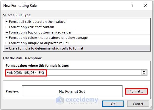
Click on Format.
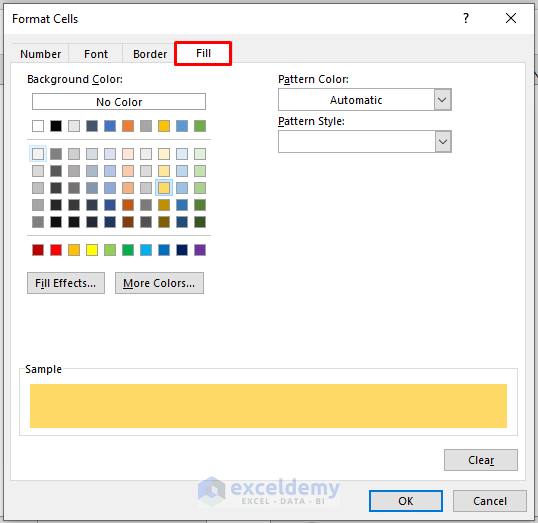
In the Format cells dialog box, selecting a color from the Fill tab.
Click on OK.

Click on OK again.
You will get the following output:

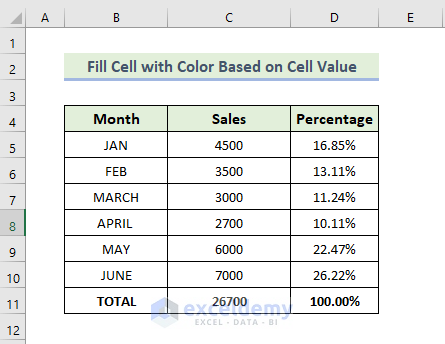
Method 2 – Fill Cells with Color Based on Cell Value in Excel

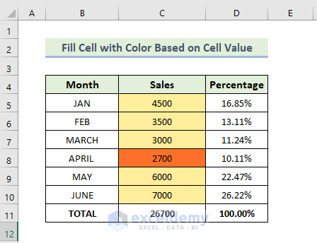
We’ll fill the cell with the lowest percentage of sales.

Steps:

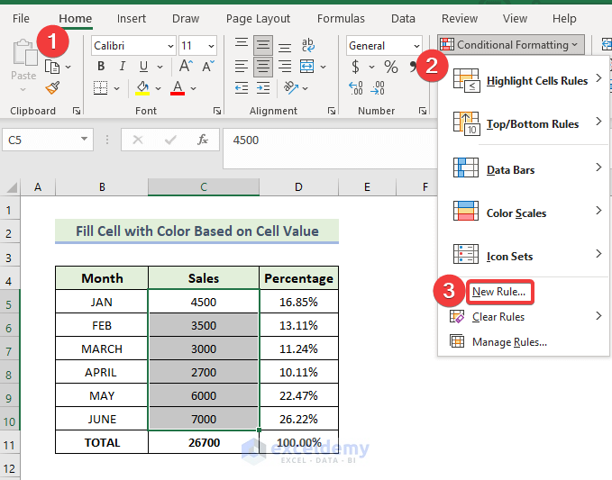
Select the range of cells C5:C10.
Go to the Home tab, select Conditional Formatting, and choose New Rule.

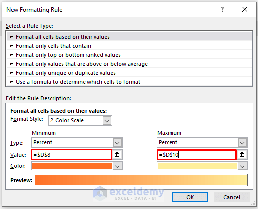
When the New formatting Rule dialog box appears, select the option Format all cells based on their values.
In the Format style option, select 2-Color Scale.
When the Minimum and Maximum option appears, select the required cell in the Value option.

In column C, cell C8 is highlighted in a different color because it has the lowest value among all cells:

Method 3 – Using Greater Than to Fill Cell with Color Based on Percentage

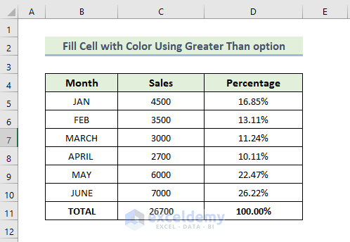
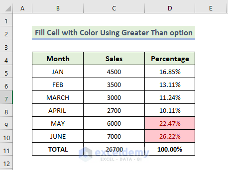
We’ll fill the cell with more than 20 percent of sales.

Steps:

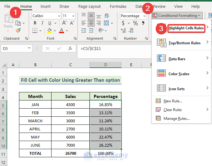
Select the range of cells D5:D10.
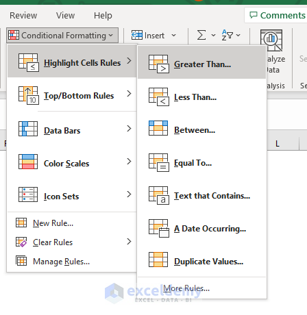
Go to the Home tab, select Conditional Formatting, and choose Highlight Cells Rules.

Select the Greater Than option.

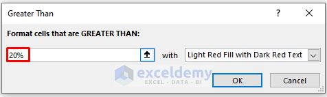
Choose the desired fill style on the right and type 20% in Format cells that are Greater Than.
Click on OK.

The cells D9 and D10 of column D are highlighted in a different color because their values are greater than 20 percent.

Method 4 – Use Text That Contains to Fill Cell with Color in Excel

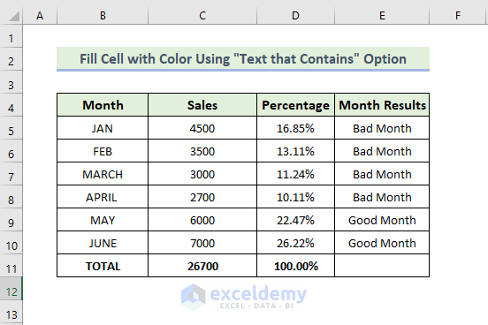
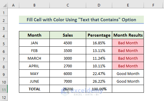
We’ll fill for cell values lower than 20%. These values have been given the designation “Bad Month” in a helper column, so we’ll use that.

Steps:

Select the range of cells E5:E10.
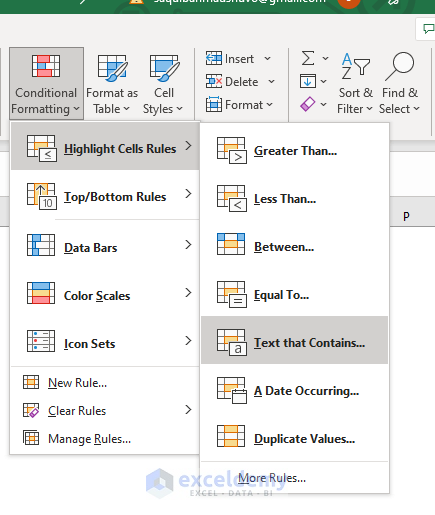
Go to the Home tab, select Conditional Formatting, and choose Highlight Cells Rules.

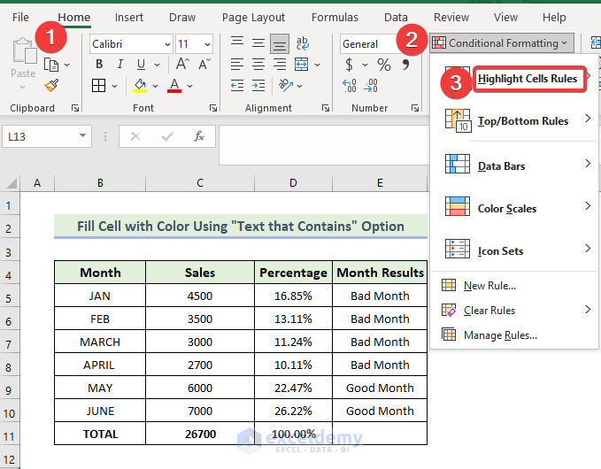
Select the Text That contains option.

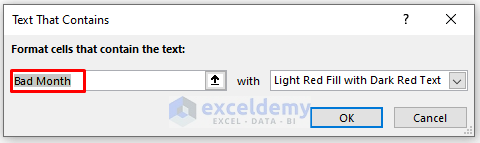
When the Text That contains dialog box appears, select the desired fill type from the right and type Bad Month in the Format cells that contain the text.
Click on OK.

The cells E5:E8 in column E are highlighted in a different color because their values are lower than 20 percent.

Method 5 – Using Top/Bottom X Rules Option

Let’s get the lowest and highest sales percentages.

Steps:

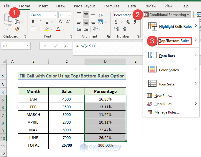
Select the range of cells D5:D10.
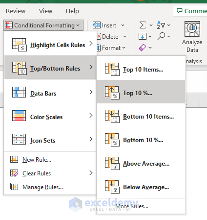
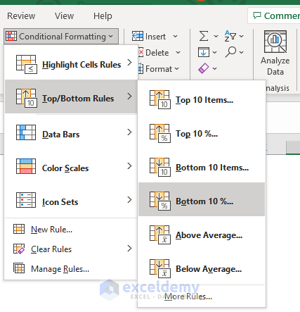
Go to the Home tab, select Conditional Formatting, and choose Top/Bottom Rules.

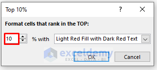
Select the Top10% option.

Select the desired fill type on the right. Leave the drop-down on 10%.
Click on OK.

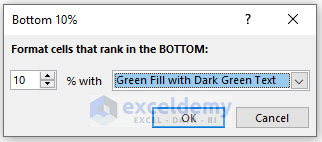
Select the Bottom 10% option if you want to get the lowest percentage value.

Choose your desired fill and click on OK.

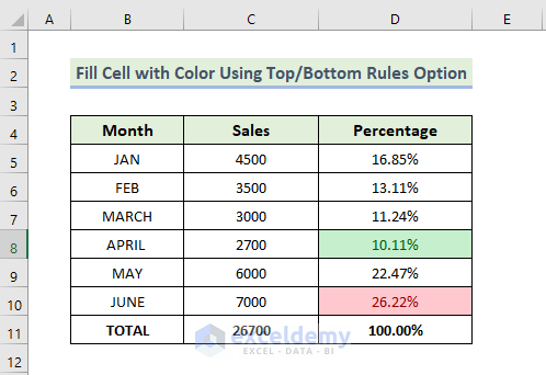
In column D, the cells D8 and D10 are highlighted in different colors because their values are the lowest and highest among all sales.

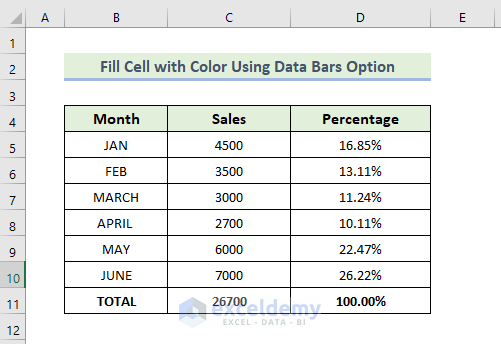
Method 6 – Fill Cells with Color Using Data Bars in Excel

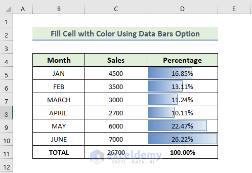
We’ll color all cells based on the percentage value.

Steps:

Select the range of cells D5:D10.
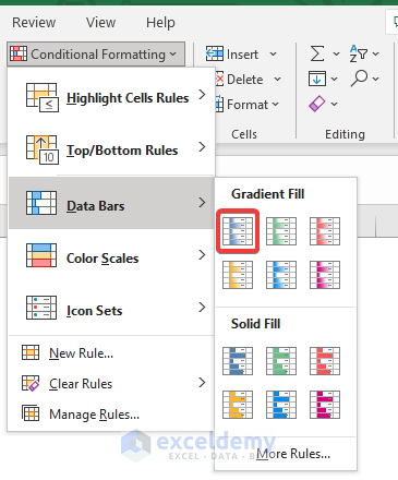
Go to the Home tab, select Conditional Formatting, and choose Data Bars.

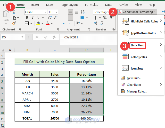
Select your desired Gradient Fill.

You will get the following output based on your criteria.

Download the Practice Workbook

Fill Cell with Color.xlsx

<< Go Back to Color Cell in Excel | Excel Cell Format | Learn Excel

Get FREE Advanced Excel Exercises with Solutions!

Sub DatabarAndConditionalFormatting() Dim lastRow As Long lastRow = ActiveSheet.Cells(Rows.Count, "B").End(xlUp).Row Dim rng As Range Set rng = Range("K2:K" & lastRow) For Each cell In rng cell.Formula = "=IFERROR(COUNTIF(B" & cell.Row & ":J" & cell.Row & ",""Yes"")/COUNTA($B$1:$J$1),0)" cell.NumberFormat = "0.00%" If cell.Value = 1 Then cell.Interior.Color = RGB(0, 255, 0) Else cell.FormatConditions.AddDatabar cell.FormatConditions(cell.FormatConditions.Count).ShowValue = True With cell.FormatConditions(1).BarColor .Color = 13012579 .TintAndShade = 0 End With End If Next cell End Sub

4 Comments

Douglas Forman Apr 28, 2023 at 2:38 AM

Is there a way to use the Data Bars then when 100% is reached the color of the cell changes? Like having a checklist that each item is either a yes or no, then when the whole row is yes?

Countif(a2:j2″yes)/counta(a1:j1)
then conditional formatting…
??
- Reply
  Lutfor Rahman Shimanto May 2, 2023 at 1:02 PM
  Hello DOUGLAS FORMAN,
  
  Thanks for reaching out and sharing your exciting query. When a given condition is met, we can use data bars and conditional formatting to change the color of a cell at a time. I can help you with Excel VBA code that loops through the K column and applies your given formula. Latterly, it utilizes an If Conditional to format each cell. When iterating, if the cell contains 1, that means 100% “Yes” It formats the fill color of the cell as Green. On the other hand, it uses a Data Bars feature. To get a better understanding of the issue, I am going to share the Workbook used in exploring your problem.
  
  Excel VBA Code:
```
Sub DatabarAndConditionalFormatting()

    Dim lastRow As Long
    lastRow = ActiveSheet.Cells(Rows.Count, "B").End(xlUp).Row
    
    Dim rng As Range
    Set rng = Range("K2:K" & lastRow)
    
    For Each cell In rng
        cell.Formula = "=IFERROR(COUNTIF(B" & cell.Row & ":J" & cell.Row & ",""Yes"")/COUNTA($B$1:$J$1),0)"
        cell.NumberFormat = "0.00%"
        If cell.Value = 1 Then
            cell.Interior.Color = RGB(0, 255, 0)
        Else
            cell.FormatConditions.AddDatabar
            cell.FormatConditions(cell.FormatConditions.Count).ShowValue = True
            
             With cell.FormatConditions(1).BarColor
                .Color = 13012579
                .TintAndShade = 0
            End With
        End If
    Next cell

End Sub
```
  INPUT: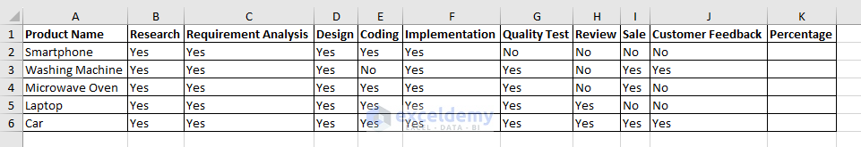
  
  OUTPUT: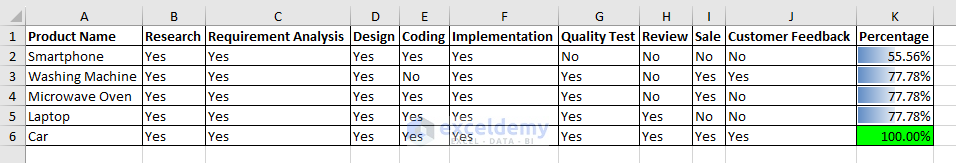
  
  WORKBOOK: Data Bars And Conditional Formatting
  
  Feel free to contact us again with any other inquiries or concerns.
  
  Regards
  Lutfor Rahman Shimanto
  ExcelDemy
sjoerd Nov 19, 2023 at 7:04 PM

can you do this with vertical databars.
or cells
I am looking to fill a cell (or better a range of cells) partially vertically (based on percentages)
See it as a tank filling with liquid
I managed to do it with sparklines in a range of cells, but then not the entire range is filled (there are white spaces on the side visible)
- Reply
  Aniruddah Alam Nov 20, 2023 at 4:40 PM
  
  Hi Sjoerd,
  
  Thanks for reaching out to us. Unfortunately, Conditional Formatting cannot create a vertical progress bar. But, using Sparkline can help you achieve your goal. You mentioned using Sparkline, but we didn’t understand what you meant by “not the entire range is filled.” Could you please clarify that?
  
  Here’s a sample picture of a vertical progress bar that we created using Sparkline.
  
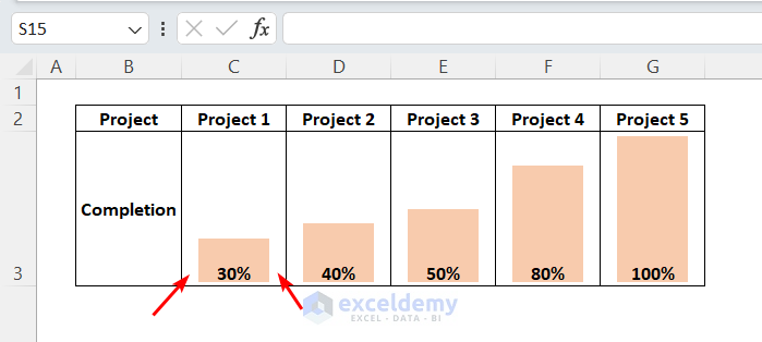
  Were you referring to the extra space on the two sides of the column, as marked in the picture? If so, we are currently unaware of any methods to eliminate the space. Please let us know your thoughts.
  
  Regards
  Aniruddah
  Team Exceldemy

How to Fill Cell with Color Based on Percentage in Excel (6 Methods)

Method 1 – Using a Formula to Fill Cell with Color Based on Percentage

Method 2 – Fill Cells with Color Based on Cell Value in Excel

Method 3 – Using Greater Than to Fill Cell with Color Based on Percentage

Method 4 – Use Text That Contains to Fill Cell with Color in Excel

Method 5 – Using Top/Bottom X Rules Option

Method 6 – Fill Cells with Color Using Data Bars in Excel

Related Articles

Leave a reply Cancel reply