Here’s an overview of the formulas we used to fill in cells with colors.
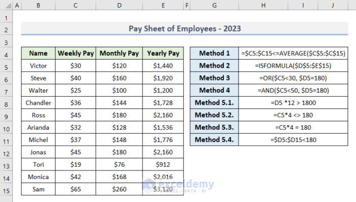
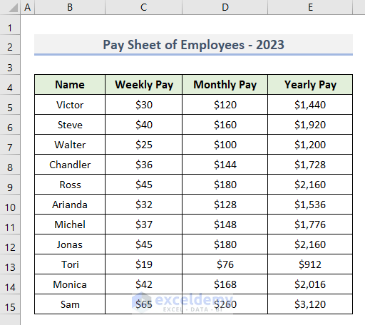
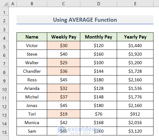
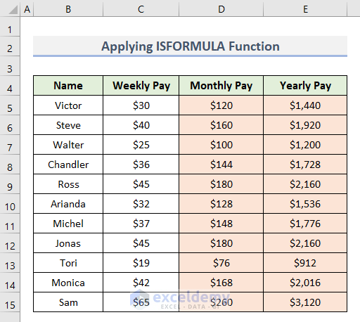
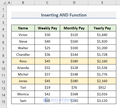
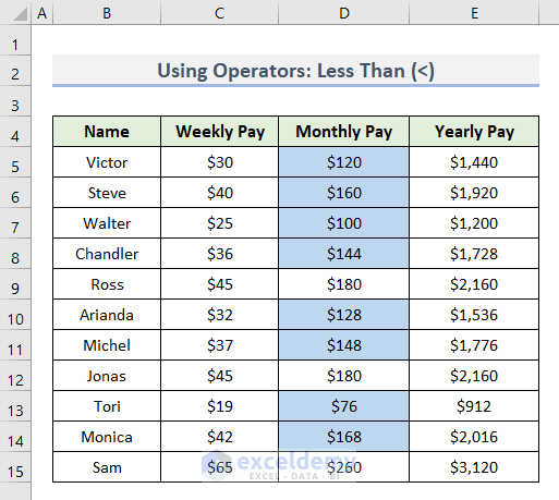
We’re using a sample Pay Sheet of several employees. There are 4 columns that represent the weekly, monthly, and yearly pay of an employee.
Method 1 – Using the AVERAGE Function with Conditional Formatting to Fill Cell Color
- Select the cell or the cell range where you want to apply this function to fill the color.
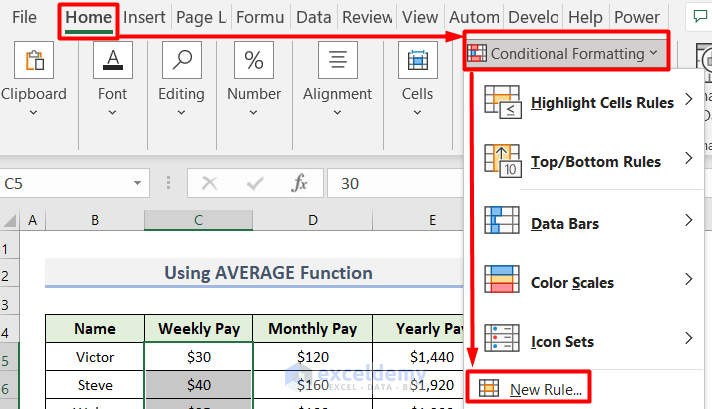
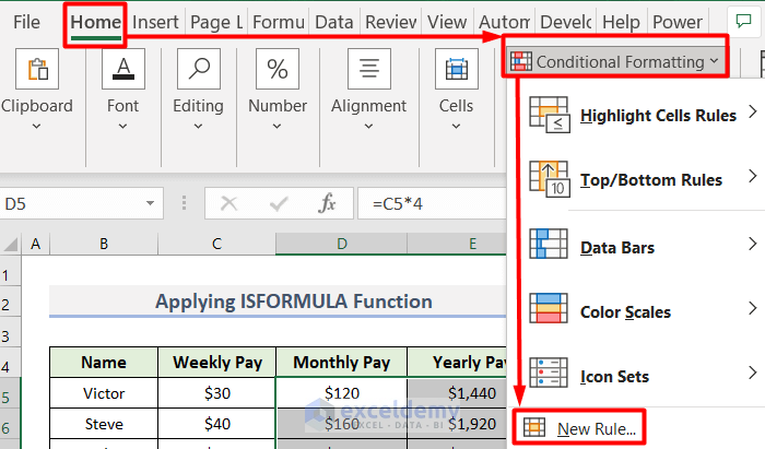
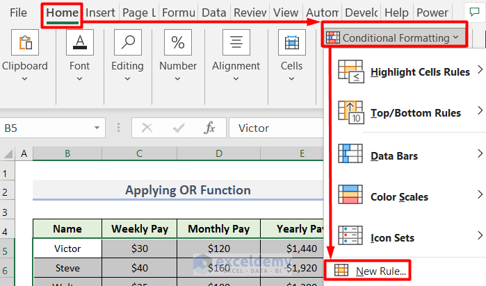
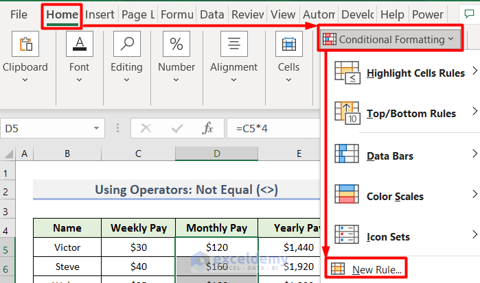
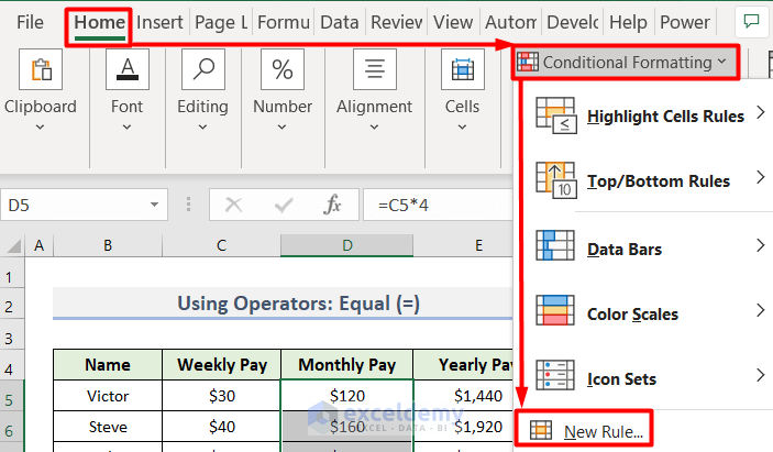
- Open the Home tab.
- Go to Conditional Formatting.
- Select New Rule.
- A dialog box will pop up.
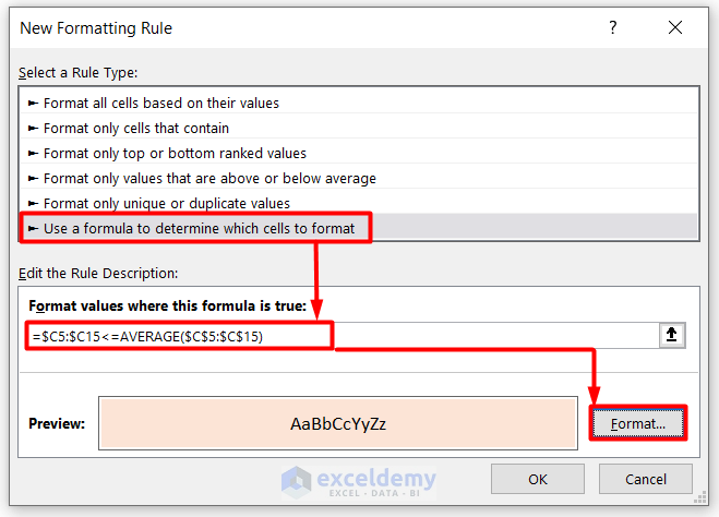
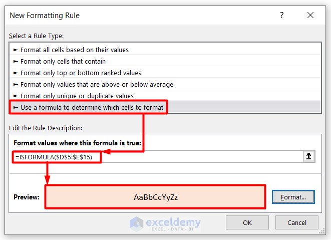
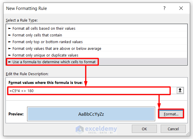
- Select Use a formula to determine which cells to format from Select a Rule Type.
- In Edit the Rule Description, insert the following formula.
=$C5:$C15<=AVERAGE($C$5:$C$15)- Click on Format.
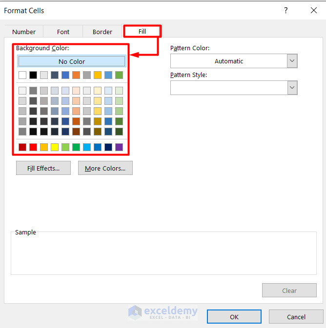
- From the Fill section, select the color of your choice to use in a cell.
- Click OK.
The AVERAGE function will calculate the average of the selected cell range C5:C15 and then will compare the average value with values of cell range C5:C15. Conditional Formatting will fill color where the cell value is less than average.
- Click OK.
Read More: Excel Formula Based on Cell Color
Method 2 – Applying the ISFORMULA Function with Conditional Formatting to Fill Cell Color
- Select the cell range where you want to fill the color using the formula.
- Open the Home tab.
- Go to Conditional Formatting and select New Rule.
- A dialog box will pop up.
- Choose Use a formula to determine which cells to format as Select a Rule Type.
- In the Edit the Rule Description, use the following formula.
=ISFORMULA($D$5:$E$15)- Go to Format and choose the color of your choice to fill color in a cell.
- Click OK.
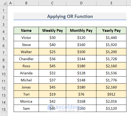
Method 3 – Fill Cell Color in Excel Using the OR Function with Conditional Formatting
- Select the cell range where you want to apply this function to fill the color.
- Open the Home tab, go to Conditional Formatting, and select New Rule.
- A dialog box will pop up.
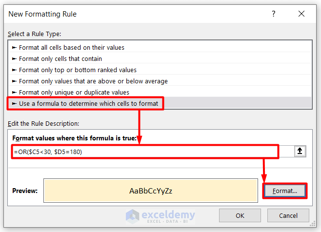
- From Select a Rule Type: select Use a formula to determine which cells to format.
- In Edit the Rule Description, use the following formula.
=OR($C5<30, $D5=180)- Select the Format of your choice to fill the color in a cell.
- Click OK.
Read More: How to Fill Cell with Color Based on Percentage in Excel
Method 4 – Using the AND Function with Conditional Formatting to Fill Cell Color in Excel
- Select the cell range to apply the AND function to fill the color.
- Open the Home tab, go to Conditional Formatting, and select New Rule.

- A dialog box will pop up.
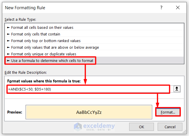
- From Select a Rule Type window, select Use a formula to determine which cells to format.
- In Edit the Rule Description, insert the following formula.
=AND($C5<50, $D5=180)- You can select the Format of your choice to fill color in a cell.
- Click OK.
Related Content: How to Change Cell Color Based on a Value in Excel
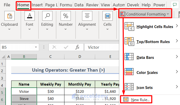
Method 5 – Highlighting Cells Based on Conditions (Greater than, Less Than, Equal to or Not Equal to)
Case 5.1 – Greater Than (>)
- Select the cell or cell range to apply the formula.
- Ppen the Home tab, go to Conditional Formatting, and select New Rule.
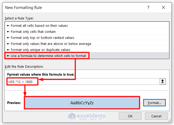
- Adialog box will pop up. From Select a Rule Type, select Use a formula to determine which cells to format.
- In Edit the Rule Description, use the following formula.
=D5 *12 > 1800- Select the Format of your choice to fill the color in a cell.
- Click OK.
- This will show the cells filled with the selected format where D5*12 is greater than 1,800.
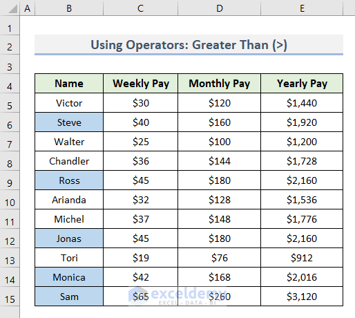
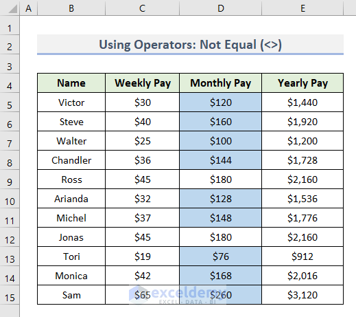
Case 5.2 – Not Equal (<>)
- Select the cell or cell range to apply the formula.
- Go to Conditional Formatting and select New Rule.
- From Select a Rule Type, select Use a formula to determine which cells to format.
- Use the following formula.
=C5*4 <> 180- From the Format option, you can select the format of your choice to fill color in a cell.
- Click OK.
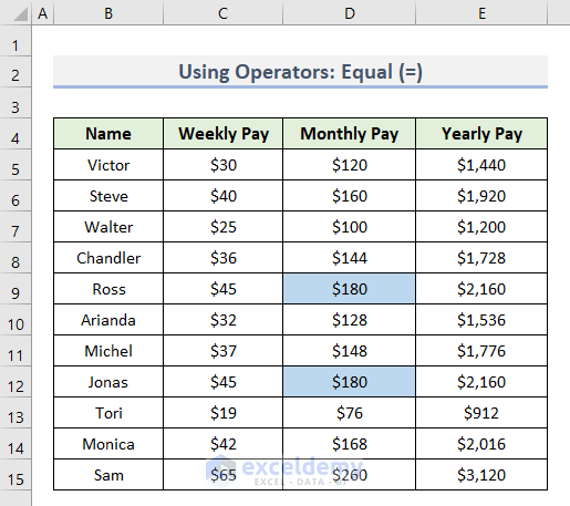
Case 5.3 – Equal to (=)
- Select the cell or cell range to apply the formula.
- Go to Conditional Formatting and select New Rule.
- A dialog box will pop up.
- Select the Use a formula to determine which cells to format rule.
- In Edit the Rule Description, use the following formula.
=C5*4 = 180- From the Format options, select the format of your choice to fill color in a cell.
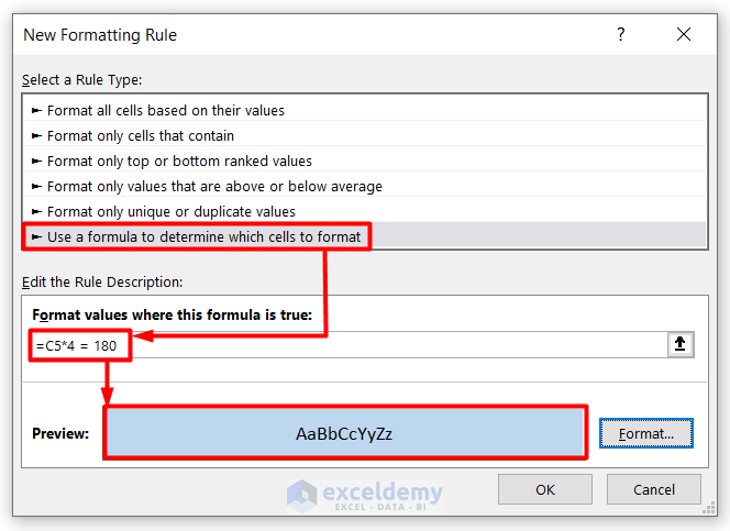
We used the (=) Equal operator to check where C5*4=180.
- Click OK.
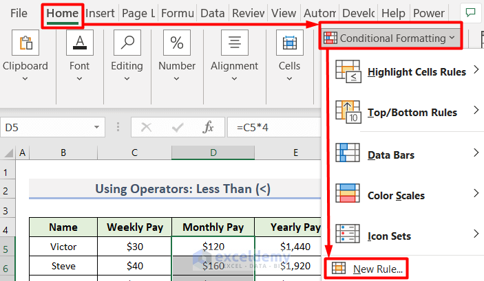
Case 5.4 – Less Than (<)
- Select the cell or cell range to apply the Less than operator.
- Go to Conditional Formatting and select New Rule.
- A dialog box will pop up.
- Select the Use a formula to determine which cells to format rule.
- Use the following formula.
=$D5:$D15<180- Select the fill color of your choice from the Format options.
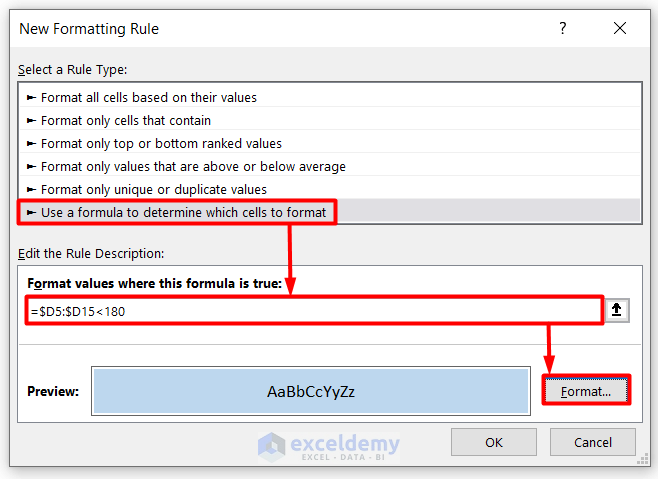
- Click OK.
Download the Practice Workbook
Related Articles
- Uses of CELL Color A1 in Excel
- How to Color Code Cells in Excel
- Excel Formula to Change Cell Color Based on Text
- VBA to Change Cell Color Based on Value in Excel
- Excel Formula to Color Cell If It Has Specific Value
- How to Change Text Color with Formula in Excel
<< Go Back to Color Cell in Excel | Excel Cell Format | Learn Excel


I have Purchased spread sheet templates and cant find where or if they have been downloaded to access
Best wishes,
Barry
Hello, Barry! You can check your default path folder for browser downloads. And if you need any assistance with the Excel problems you can mail us!