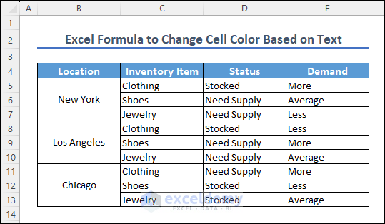
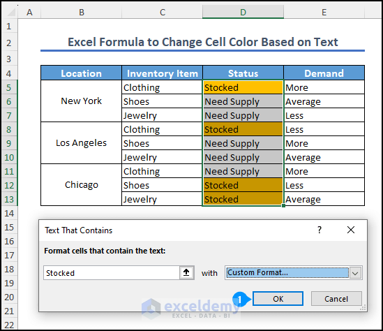
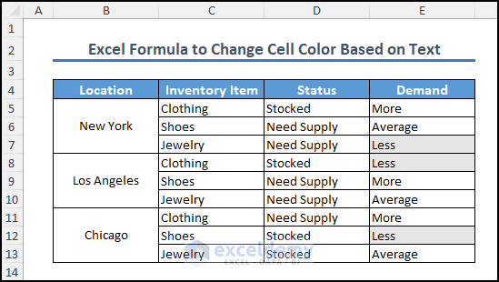
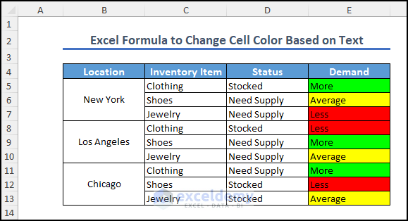
Excel Formula to Change Cell Color Based on Text (3 Easy Methods)

Suppose you have the following dataset:

Method 1 – Applying Conditional Formatting

Steps:

Application of Cell Rules

Select the data range containing the cells you want to format (D5:D13 in this example).

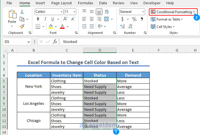
Go to the Home ribbon and find the Conditional Formatting drop-down arrow in the Styles group.
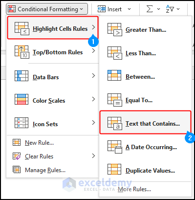
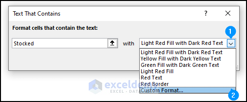
From the menu, select Highlight Cells Rules and choose Text that contains….

In the left box of the small window that appears, type or select the text you want to format (Stocked).

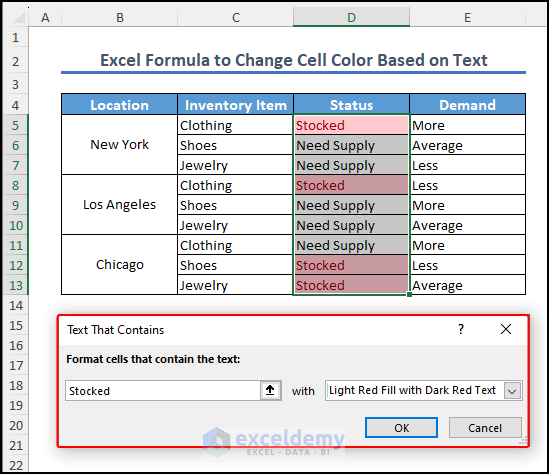
In the right box, select the color you want to use by clicking the down arrow. There are a few built-in options. but select Custom Format.

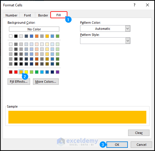
The Format Cells window will open automatically. Click the Fill tab and select the orange color.
Click OK.

Preview the changes and make any changes necessary.
Click OK.

Repeat the steps above to apply formatting for any additional text.
Preview the changes and make any changes necessary.
Click OK.

Creating New Rules

Select the data range for the demand column (column E).
Go to the Home ribbon and click on Conditional Formatting in the Style group.

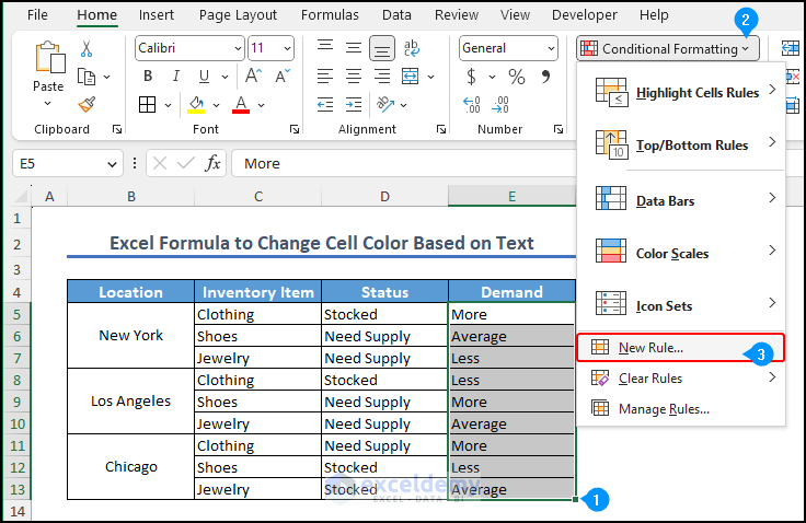
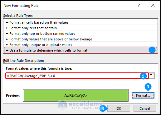
From the drop-down menu, choose New Rule. The New Formatting window opens.
Select the Use a formula to determine which cells to format option.
In the input box, enter the following formula:

=SEARCH("Less",E5:E13)>0

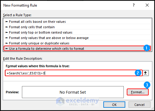
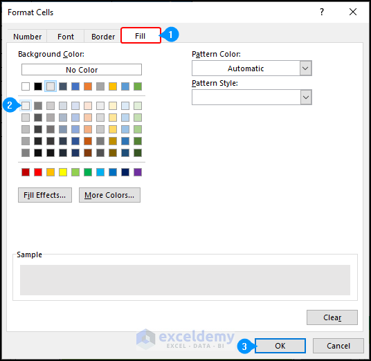
Click on the Format button. In the Format Cells dialog box, go to the Fill tab and choose the appropriate color.
Click OK to apply the formatting and close the dialog box.

Preview the changes in the preview box.

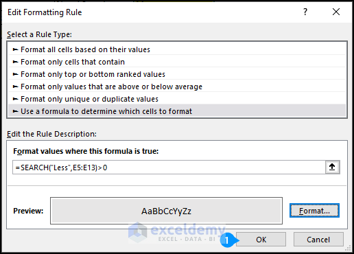
Click OK.

Repeat the same process for the remaining text (Average and More). For the text Average in this example, select the light green color for formatting and use the following formula:

=SEARCH("Average",E5:E13)>0

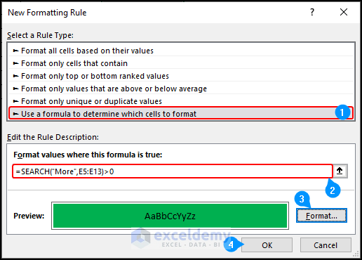
Repeat for the text More, with the formula below:

=SEARCH("More",E5:E13)>0

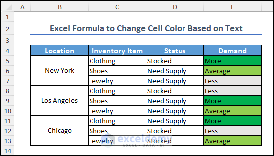
Preview the changes and make any changes necessary.

Method 2 – Employing VBA Code

Steps:

Select the cells you want to include in the range (E5 to E13).
Go to the Formulas tab and choose Define Names from the Define Name drop-down menu.

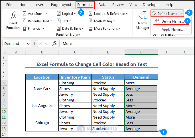
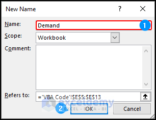
When a window opens, name the range (Demand).
Click OK.

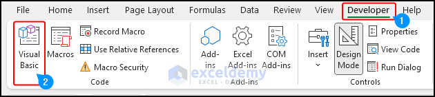
Go to the Developer tab and choose Visual Basic.

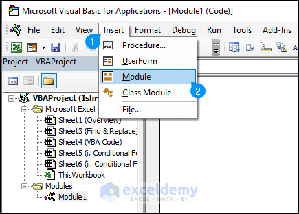
In the VBA window, click Insert and then select Module.

Enter the following code and save it:

Sub Fill_Color()
Dim cell_value As Range
Dim stat_value As String
Dim rng As Range
Set rng = Range("Demand")
For Each cell_value In rng
stat_value = cell_value.Value
Select Case stat_value
Case "More"
cell_value.Interior.Color = RGB(0, 255, 0)
Case "Average"
cell_value.Interior.Color = RGB(255, 255, 0)
Case "Less"
cell_value.Interior.Color = RGB(255, 0, 0)
End Select
Next cell_value
End Sub

Code Breakdown:

The code creates a Sub procedure named Fill_Color.
After declaring variables, The Set rng = Range(“Demand“) line sets the variable rng to refer to the range named “Demand” in the worksheet. This range will be the target for the color formatting actions performed in the code.
The Select Case statement is used to evaluate the value of the variable stat_value. It allows different code blocks to be executed based on the value of stat_value.
In this example, there are three cases: “More”, “Average”, and “Less”. Each case represents a specific value that stat_value can take. Depending on the value of stat_value, the corresponding code block is executed.
Inside each code block, the Interior.Color property of the current cell (cell_value) is set to a specific RGB color value. This effectively changes the cell’s background color based on the value of stat_value.
“End Select” marks the end of the Select Case statement. “Next cell_value” indicates that it moves to the next cell in the range and continues the loop.

Click Run or go to Macros under the Developer tab and choose the code you just created.

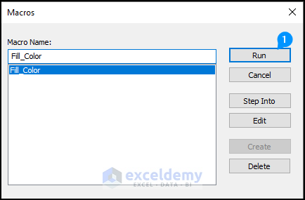
The cells now have fill colors based on the text they contain.

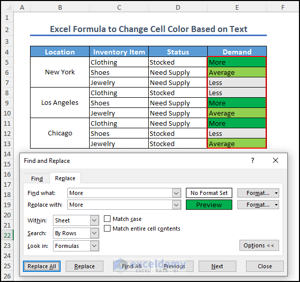
Method 3 – Change Cell Color Based on Text: Excel Find and Replace Tool

Steps:

Press Ctrl + H or go to the Home ribbon and select the down arrow of the Find and Replace menu from the Editing group.
Click Replace to open the find and replace dialogue box.

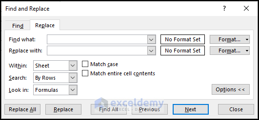
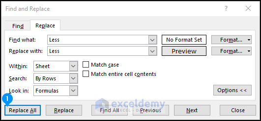
In the Find what box, type the text you want to highlight (Less), and in the Replace with box, type the same text.
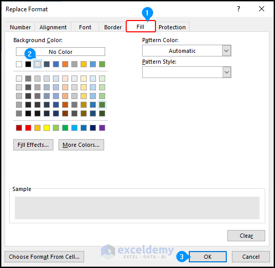
To the right of the Replace with row, click Format to open the options.

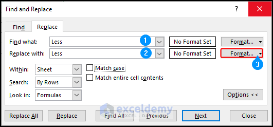
Go to the Fill option and select the appropriate color from the Replace Format box.
Preview the color in the sample box.
Click OK.

Click the Replace All button.

A notification window will pop up with the number of replacements.

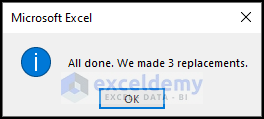
Without closing the find and replace menu, view the changes.

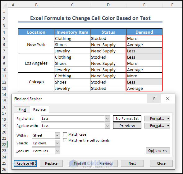
Repeat the same process for all the other text.
Preview the changes and once everything is correct, close the Find and Replace menu.

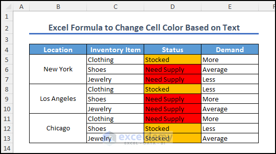
The finished formatting should look similar to the image below:

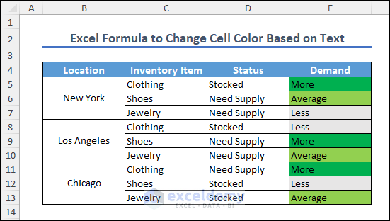
NOTE: When using the Find and Replace tool to highlight cells, the fill color remains consistent even if the cell values change. Cell color will have to be manually changed.

Things to Remember

When using conditional formatting for specific text, you need to repeat the process for each unique text individually.
In addition to using functions, you can also directly refer to cells in conditional formatting.
Using VBA code is the shortest and easiest method to apply Excel formulas to change cell color based on text.

Frequently Asked Questions

How can I remove conditional formatting from a cell in Excel?

Select the cell and go to Conditional Formatting in the “Home” tab. Choose Clear Rules and select Clear Rules from Selected Cells.

Can I use an IF statement to change cell color in Excel?

No, an IF statement cannot directly change the color of a cell in Excel. However, you can use an IF statement in conditional formatting to determine when to apply a specific color to a cell.

What are the different conditional formatting options in Excel?

The main conditional formatting options in Excel are:

Highlight Cell Rules: It highlights cells based on specific criteria.
Top/Bottom Rules: For highlighting the top or bottom values in a range.
Data Bars, Color Scales, and Icon Sets: if you want to add visual indicators to cells.

Can I use a custom color for a cell based on its text value?

Yes. In the Conditional Formatting dialog box, select “Custom Format,” go to the “Fill” tab, and choose a custom color for the cell.

How can I change the font color based on the cell value in Excel?

Select the cells, go to the Home tab, and click on Conditional Formatting. Then choose Highlight Cells Rules and Text that Contains. Enter the text value and select the custom format option and go to the Font menu from the Formatting cell dialogue box. Select the font color to apply.

Download Practice Workbook

You can download the workbook, where we have provided a practice section on the right side of each worksheet. Try it yourself.

Formula to Change Cell Color Based on Text.xlsm

Get FREE Advanced Excel Exercises with Solutions!

Excel Formula to Change Cell Color Based on Text (3 Easy Methods)

Method 1 – Applying Conditional Formatting

Method 2 – Employing VBA Code

Method 3 – Change Cell Color Based on Text: Excel Find and Replace Tool

Things to Remember

Frequently Asked Questions

Download Practice Workbook

Related Articles

Leave a reply Cancel reply