Latest Posts From Ishrak Khan

In this article, we will review the benefits of using the print scale in Excel. The ability to scale prints is crucial for professionals who rely on Excel for ...

The F test is used to determine if two sample groups have similar variances. Download Practice Workbook Download the workbook. F Test.xlsx ...

List of Excel Statistical Functions: AVERAGE Function MEDIAN Function MODE Function STDEV Function VAR Function COUNT Function MIN ...

In this article, we have demonstrated all the necessary information that is related to Excel unique values. We will use functions and pivot table to ...

In Excel, cell styles offer a wide range of professionally designed formats which enable applying a uniform, visually appealing look to worksheets quickly and ...

Excel Information Functions: Knowledge Hub CELL Function IFERROR Function ISBLANK Function ISERROR Function ISEVEN Function ISLOGICAL ...

Here's an overview of the Print menu in Excel. You can choose your printer, and you can change print settings including what to print, how many copies to ...

When you open an Excel workbook, the grid-like faint gray lines presenting the cells, rows, and columns are formally known as Excel Gridlines. In this Excel ...
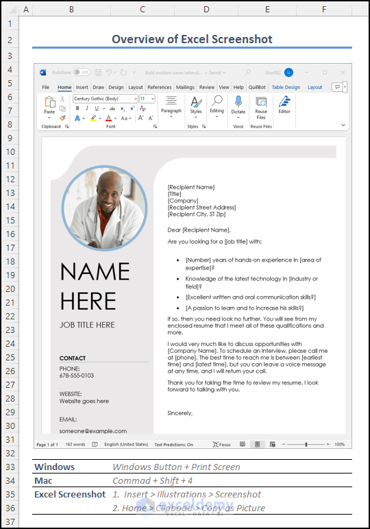
To take a screenshot in Excel, first, go to the Insert tab and then select the Screenshot option from the Illustrations group. There are two options ...
Method 1 - Format Data Structure for Waterfall Chart We will use a financial dataset that includes two products (A & B), each with quarterly income and ...

This is an overview. Download Practice Workbook Download the workbook and practice. Range Address.xlsm Syntax of the Excel VBA Range ...
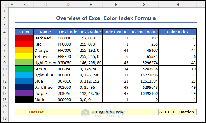
In this article, we will explain how to use the Excel color index formula. One of the standout features of Excel Color Index is its extensive ...

This article will demonstrate how to add and utilize an Excel button tooltip to enhance the accessibility and user-friendliness of complex spreadsheets. In our ...
![[Solved!] MINVERSE in Excel Not Working](https://www.exceldemy.com/wp-content/uploads/2023/07/1-overview-image-of-minverse-excel-not-working.png?v=1697522321)
Here's an image overview of the most common reasons behind the MINVERSE function not working properly. Download the Practice Workbook MINVERSE ...
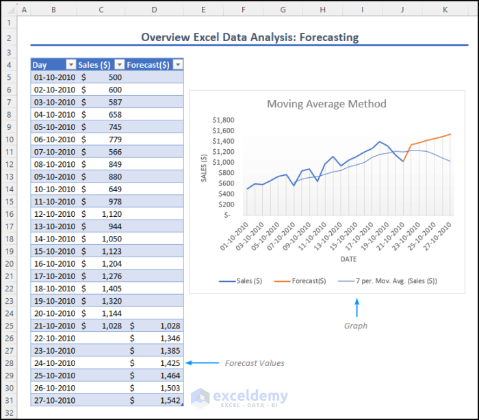
Download Practice Workbook Data Analysis Forecast.xlsx Method 1 - Using Moving Average Method for Forecasting Data Analysis in Excel 1.1 Using ...
See Our Reviews at


Dear MATHMAN,
We are glad that you have already got your answer related to the ROUND function.
Now let’s jump to the problem related to finding other EigenValue and EigenVector using the power method.
In the power method, it is a must to choose an initial vector V0. So, the tips for what to keep in mind while randomly choosing an initial vector V0:
If initial vector V0 =[0,1,1] and W is the given dominant Eigenvector, then V0 X W =0
The dominant Eigenvalue for the 3×3 matrix [5,4,-1; 4,5,1; -1,1,2] is approximately λ ≈ 9.
If you are getting Eignevalue λ≈0 for the initial EigenVector V0 = [0,0,1] most probably because the vector has no magnitude along the x and y axes and a magnitude of 1 along the z-axis. Therefore, the initial vector V0 does not converge to the dominant Eigenvalue for the given matrix. It is expected that different EigenVectors can lead to different EigenValues.
The dominant eigenvalue is typically the one with the largest magnitude. It is recommended to use multiple initial vectors in the power method so that you know which eigenvalue converges to the dominant eigenvalue.
I hope this solution resolves your issue. Feel free to email us at [email protected] if you have any further problems or inquiries.
Regards,
Qayem Ishrak Khan
Team ExcelDemy.
Dear ALEX,
Thank you for this interesting question. If you want to find the total sales value for each brand within a quarter or QTD, you can use a formula that combines the SUMIFS, INDEX, and MATCH functions.
Formula:
=SUMIFS(INDEX(D5:I14,0,MATCH(D16,D4:I4,0)),B5:B14,D17,C5:C14,D18)+SUMIFS(INDEX(D5:I14,0,MATCH(E16,D4:I4,0)),B5:B14,D17,C5:C14,D18)+SUMIFS(INDEX(D5:I14,0,MATCH(F16,D4:I4,0)),B5:B14,D17,C5:C14,D18)The formula used here is the same as the one explained in the “Use of SUMIFS with INDEX & MATCH Functions in Excel” section. We repeat the formula two more times, adjusting the column reference for each specific month in the quarter.
I hope this solution resolves your issue. Feel free to email us at [email protected] if you have any further problems or inquiries.
Regards,
Qayem Ishrak Khan
Team ExcelDemy.