How to Change Text Color with Formula in Excel (2 Methods)

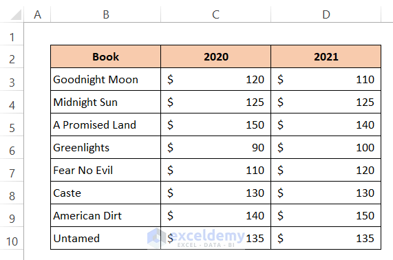
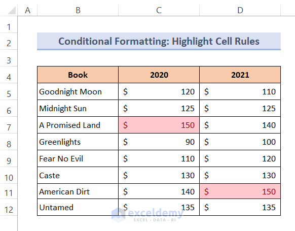
We have some book names and their online prices for two consecutive years. We’ll change the color of the prices with the formula.

Method 1 – Formula with Conditional Formatting to Change Text Color in Excel

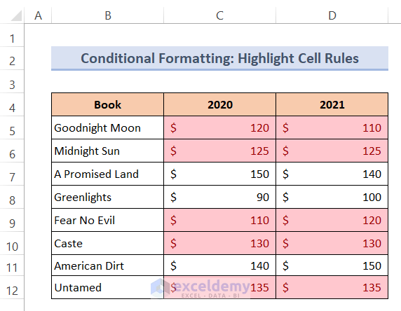
Case 1.1 – Use Highlight Cells Rules

Steps:

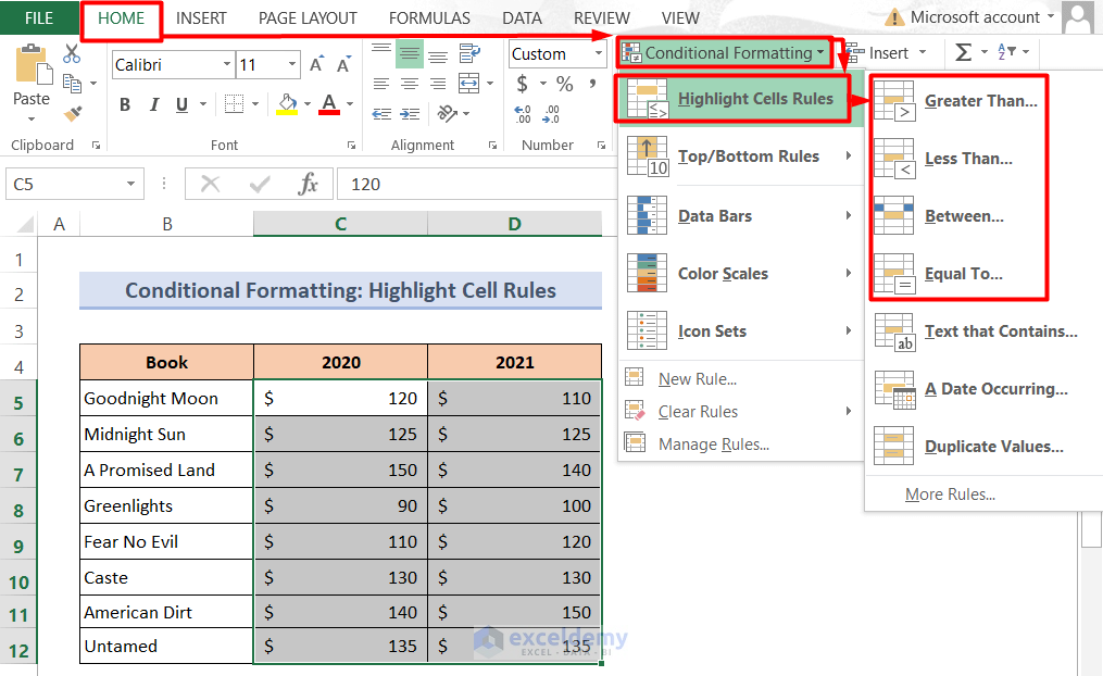
• Select the data range C5:D12.
• Go to Home, then select Conditional Formatting and choose Highlight Cells Rules.
• You will get 4 options: Greater Than, Less Than, Between, and Equal To.
• Select which one you need.

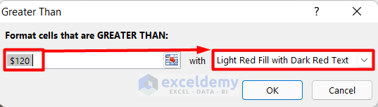
Steps for Greater Than:

• Select your desired range in Format cells that are GREATER THAN box.
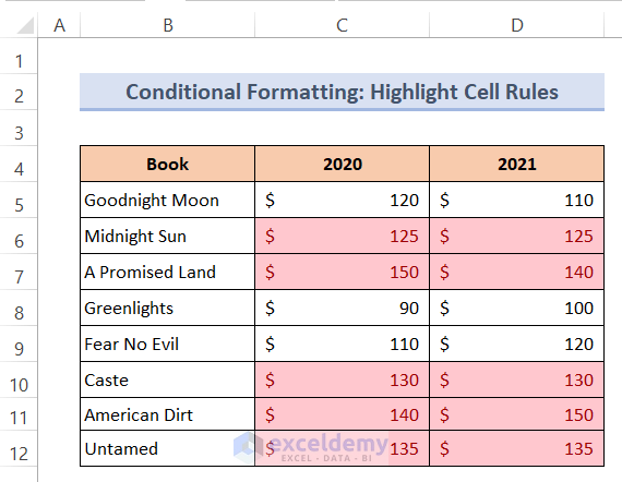
• We have set the value at $120. Excel will change the color of the text and highlight only those values that are greater than $120.
• Select your desired color.
• Press OK.

• Here are the results.

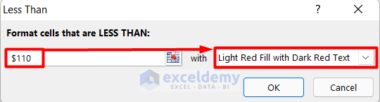
Steps for Less Than:

• We have set the less than the value at $110. That means it will change the color of the text and highlight only those values that are less than $110.
• Select your desired color.
• Press OK.

• Here are the results.

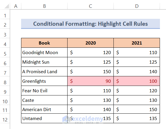
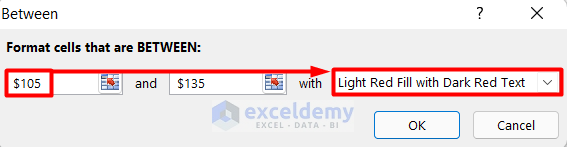
Steps for Between:

• Set the start and end range values in their respective boxes.
• Select your desired color.
• Press OK.

• Here’s our output:

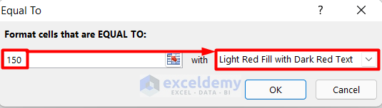
Steps for Equal To:

• Set the value in the Format cells that are EQUAL TO box.
• Select a color.
• Press OK.

• Here are the results.

Case 1.2 – Apply New Rule

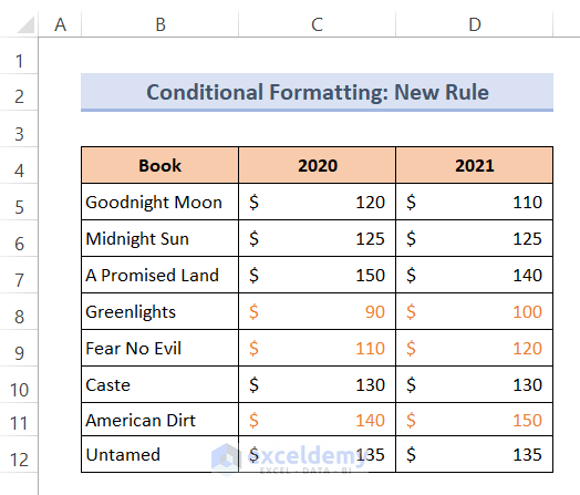
We’ll change the text color of those rows if the values in Column C are greater than Column D.

Steps:

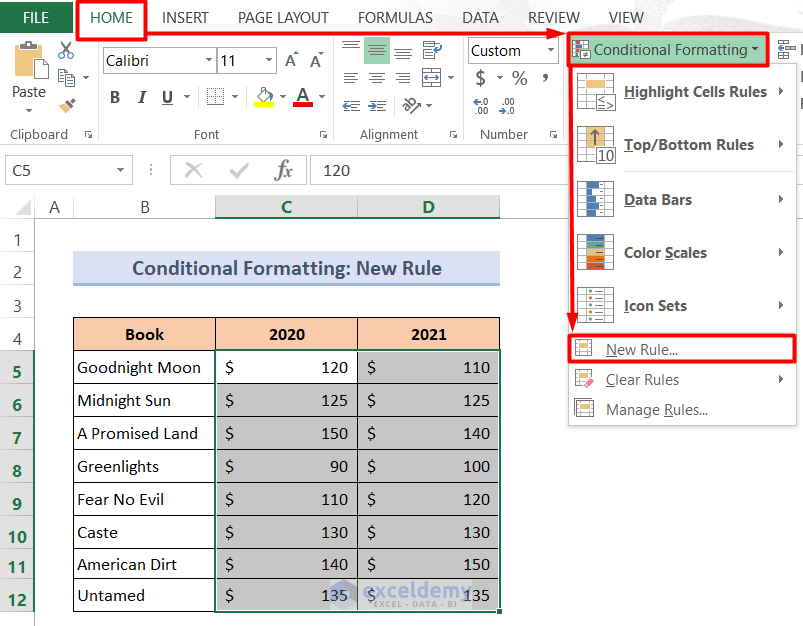
• Select the data range C5:D12.
• Go to Conditional Formatting and choose New Rule.
• A dialog box will appear.

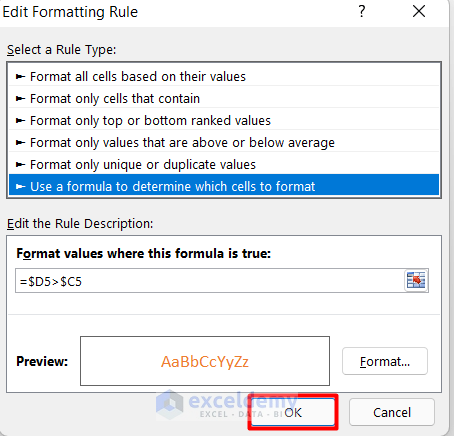
• Select Use a formula to determine which cells to format under Select a Rule Type.
• Use the formula given below in Format values where this formula is true box.

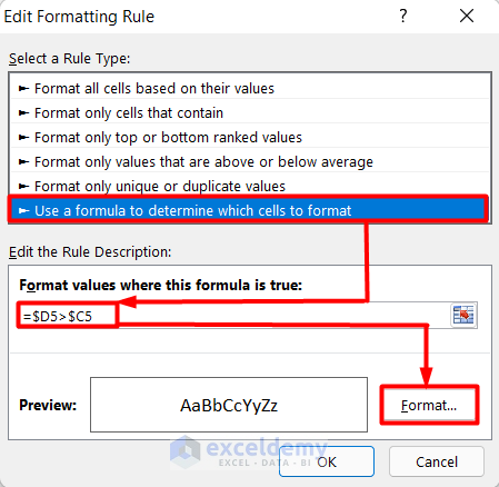
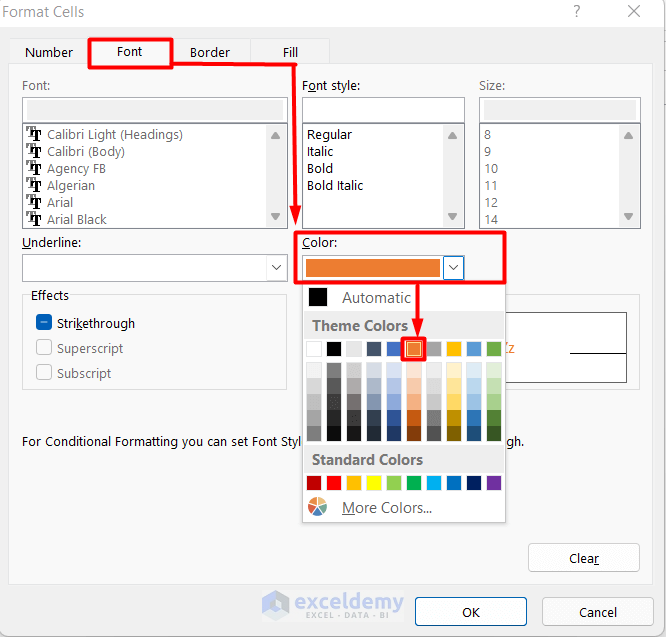
• Press Format. Another dialog box will open up.
• Set your desired color from the Color box of the Font option. You can also choose a Fill color instead from the Fill tab.
• Press OK.

• Press OK again.

• Here’s our output with the picked text color.

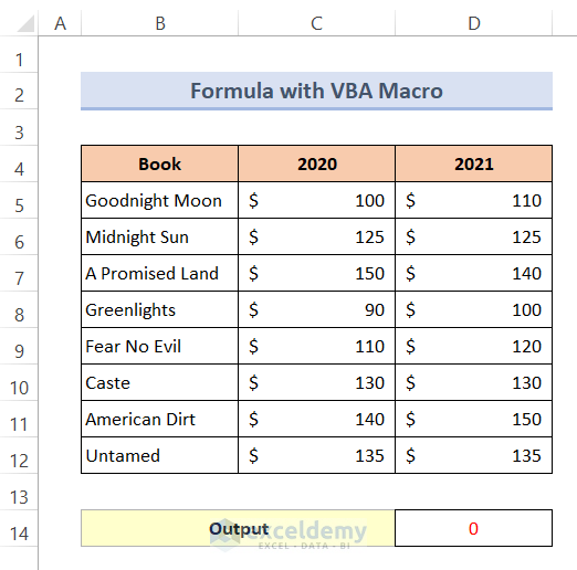
Method 2 – Using VBA Macros to Change Text Color in Excel

Steps:

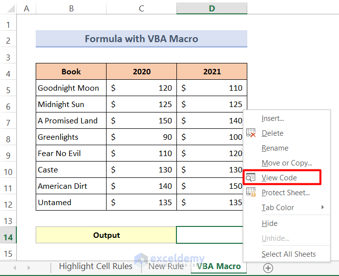
• Right-click on the sheet title.
• Select View Code from the context menu.
• A VBA window will open up.

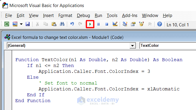
• Insert the code given below:

Function TextColor(n1 As Double, n2 As Double) As Boolean
    If n1 <= n2 Then
        Application.Caller.Font.ColorIndex = 3
    Else
        ' Set font to normal
        Application.Caller.Font.ColorIndex = xlAutomatic
    End If
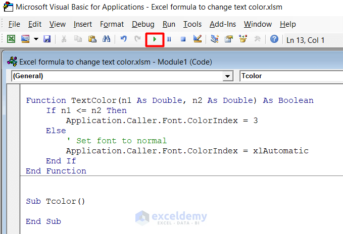
End Function
Sub Tcolor()
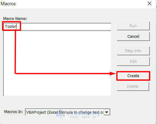
End Sub

• Press the Run icon. You’ll get a new dialog box to create a macro.

• Give the macro a name.
• Press Create.

• Press the Run icon again to run the codes.

• Insert the following formula in Cell D14:

• Hit the Enter button.

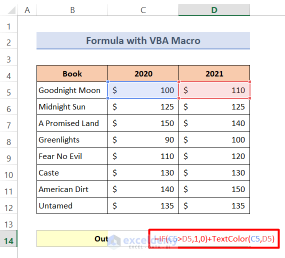
• Here’s the result.

Download the Practice Book

Related Articles

• Uses of CELL Color A1 in Excel
• How to Color Code Cells in Excel
• Excel Formula to Change Cell Color Based on Text
• How to Change Cell Color Based on a Value in Excel
• How to Fill Color in Cell Using Formula in Excel
• How to Fill Cell with Color Based on Percentage in Excel
• Excel Formula to Color Cell If It Has Specific Value
• How to Apply Formula Based on Cell Color in Excel
• VBA to Change Cell Color Based on Value in Excel

<< Go Back to Color Cell in Excel | Excel Cell Format | Learn Excel