Method 1 – Use Conditional Formatting to Highlight Row Based on Criteria
Steps to Apply Conditional Formatting Using Custom Formula:
- Select the dataset that consists of the rows to highlight.
- Go to the Home tab. Then look for the Styles group.
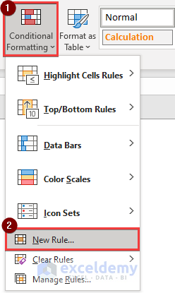
- Click the Conditional Formatting button, and the following drop-down list will appear.
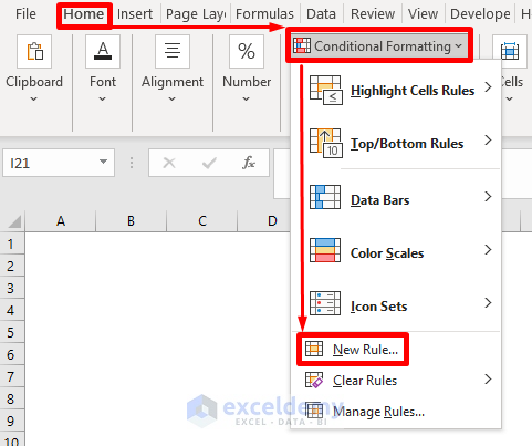
- Press the New Rule button, and the following window will appear.
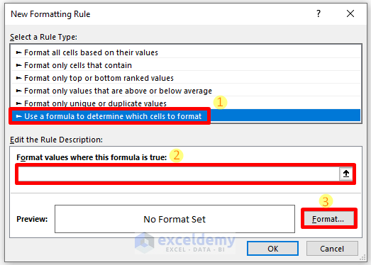
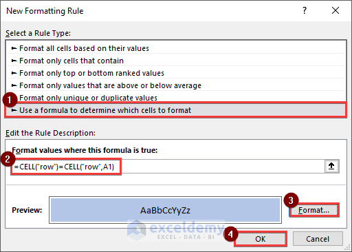
- Select “Use a formula to determine which cells to format” as Rule Type.
- Type a suitable formula in the box named “Format values where this formula is true:“.
- Click the Format button.
You will see the following window, named “Format Cells“.
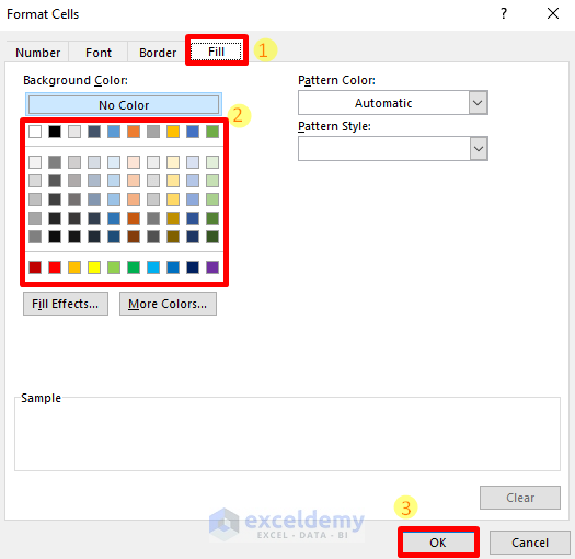
- Go to the Fill tab and select a suitable background color.
- Press OK.
The following window will appear again this time.
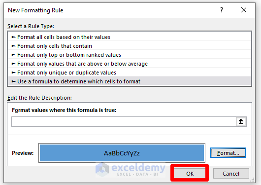
- Press OK.
In the following subsections, we will provide certain formulas highlighting rows based on different criteria.
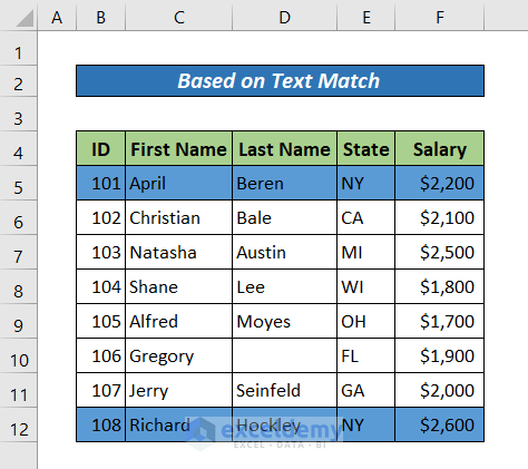
Criteria 1: Based on Text Match
Criteria:
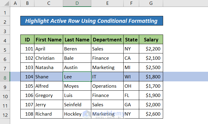
Our goal is to highlight all the rows where the state name is “NY“.
Formula to Apply:
=$E5="NY"
Result:
Criteria 2: Based on Number Match
Criteria:
Our goal is to highlight all the rows having a salary greater than 2000.
Formula to Apply:
=$F5>2000
Result:

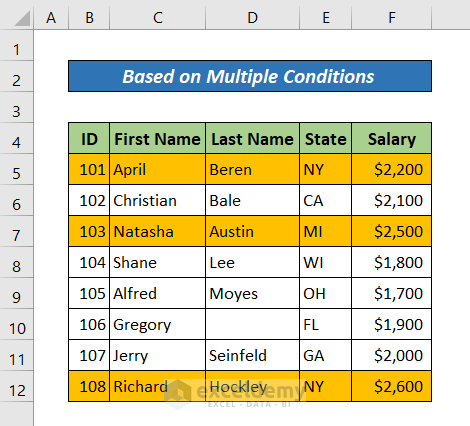
Criteria 3: Based on Multiple Conditions
Criteria:
We aim to highlight all rows containing either ‘MI’ or ‘NY’.
Formula to Apply:
=OR($E5="MI",$E5="NY")
Result:
We must highlight a row containing the first name ‘Jerry’ and state ‘GA’.
The formula will be,
=AND($C5="Jerry",$E5="GA")Criteria 4: If Row Contains Blank Cells
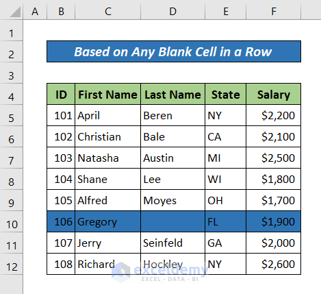
Criteria:
Our goal is to find if there is any blank cell in a row. If found, then highlight it.
Formula to Apply:
=COUNTIF($B5:$F5,"")>0“” denotes blank
Result:
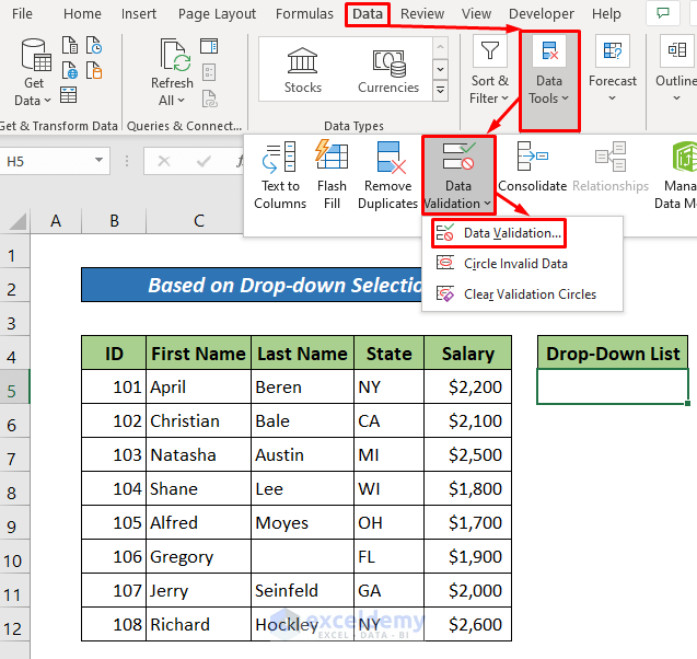
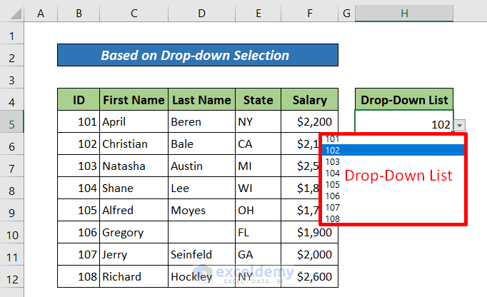
Criteria 5: Based on Drop-Down Selection
Follow the steps below to dynamically highlight a row by selecting a name from the drop-down selection list.
Creating a Drop-Down List:
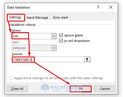
- To create a drop-down list, select a cell (H5 in this example). Go to the Data tab. From the Data Tools group, click on the Data Validation drop-down and the Data Validation option. A Data Validation box will pop up.
- After selecting List as the validation criteria, a source field will appear. In the Source box, enter the following formula
=$B$5:$B$12- Press OK.
A drop-down list is created in Cell H5 now.
Applying Conditional Formatting:
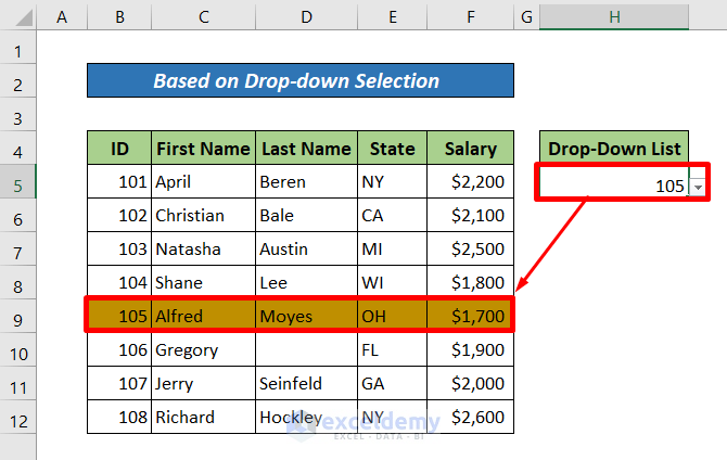
Now, apply Conditional Formatting as described at the very beginning with the following formula.
Formula to Apply:
=$B5=$A$3Select an option from the drop-down list you have created, the row that contains it will be highlighted automatically.
Result:
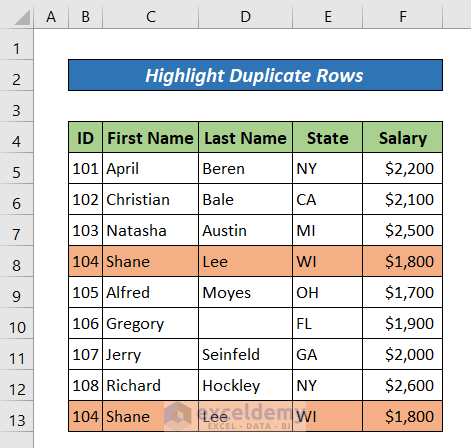
Criteria 6: Highlight Duplicate Rows
Formula to Apply:
=COUNTIF($B$5:$B$13,$B4,$C$5:$C$13,$C4,$D$5:$D$13,$D4,$E$5:$E$13,$E4,$F$5:$F$13,$F4)>1Where,
→ $B$5:$B$13, $C$5:$C$13, $D$5:$D$13, $E$5:$E$13, $F$5:$F$13 are the ranges.
→ $B4, $C4, $D4, $F4 are the criteria.
Result:
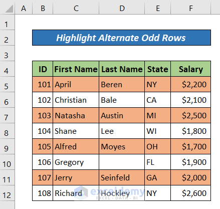
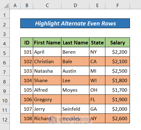
Criteria 7: Highlight Alternate Rows
Formula to Apply:
For odd rows,
=ISODD(ROW())For even rows,
=ISEVEN(ROW())Result:
Highlighted alternate odd rows-
Highlighted alternate even rows-
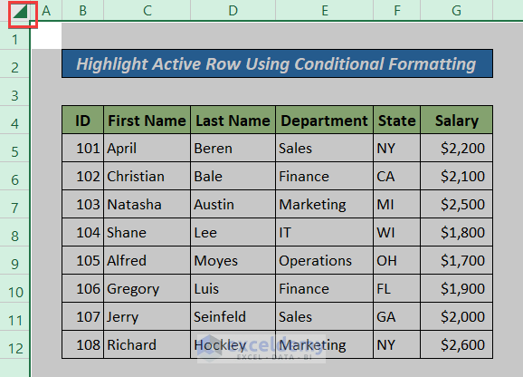
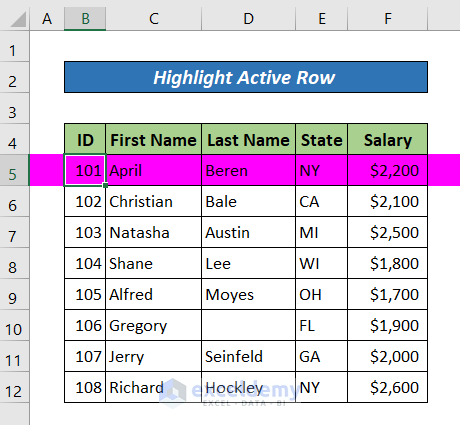
Criteria 8: Highlight Active Row
- Select the entire worksheet using Ctrl+A or click on the top left corner of the sheet.
- Go to Home >> Conditional Formatting and select New Rule.
- Open the New Formatting Rule window.
- Select Use a formula to determine which cells to format option from the Select a Rule Type
- Insert the following formula in the Format values where this formula is true
=CELL("row")=CELL("row",A1)
The CELL function returns the row number of a specific or active cell.
- Click on the Format button and choose the color of your preference.
- Click OK.
- Click on any cell in the dataset, and the whole active row will be highlighted.
Method 2 – Highlight an Active Row Using Excel VBA
Steps:
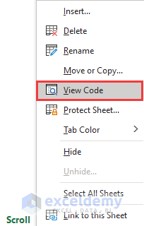
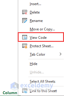
- Do Right-click on the Sheet name (VBA in this example) where you need to highlight the active row. Click the View Code.
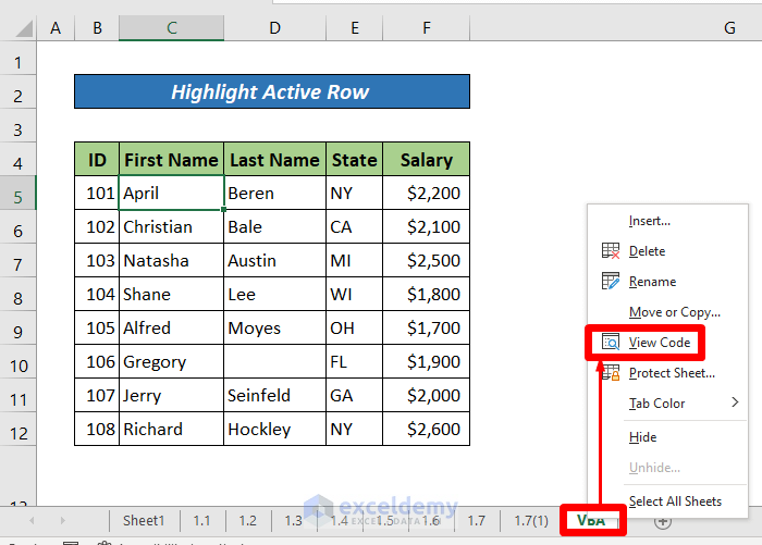
- A VBA window will pop up. Type the following code in the Code window.
Sub Worksheet_SelectionChange(ByVal Target As Excel.Range)
Static mRow
If mRow <> "" Then
With Rows(mRow).Interior
.ColorIndex = xlNone
End With
End If
Active_Row = Selection.Row
mRow = Active_Row
With Rows(Active_Row).Interior
.ColorIndex = 7
.Pattern = xlSolid
End With
End Sub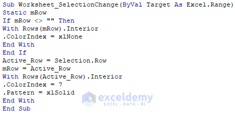
Change the highlighting color by changing the ColorIndex number.
- Close the VBA window.
Select a cell in the worksheet, the whole corresponding row will be highlighted.
Method 3 – Highlight Active Row While Scrolling
- Right-click on the sheet name to select View code.
- Insert the following VBA code.
Private Sub Worksheet_SelectionChange(ByVal SelectedRange As Range)

    Cells.Interior.Color = RGB(255, 255, 255) ' Sets the fill color to white

    SelectedRange.EntireRow.Interior.Color = RGB(0, 255, 255) ' Sets the fill color to cyan

End Sub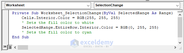
This line Private Sub Worksheet_SelectionChange(ByVal SelectedRange As Range) declares the event Worksheet_SelectionChange, it activates when the selection changes in the worksheet.
- Scroll using the down arrow on the keyboard. The code will highlight the active row while scrolling.
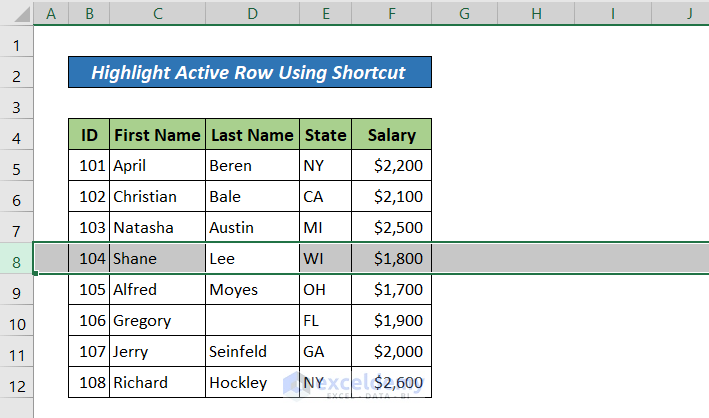
Method 4 – Shortcuts to Highlight Row in Excel
| Task | Shortcut |
|---|---|
| Highlight Active Row | Select a cell in the row >> Shift + Spacebar |
| Highlight an Entire Row | Click on the row number |
| Highlight Non-Adjacent Cells | Select the first cell >> Hold Ctrl key >> Select the last cell |
| Highlight the Entire Worksheet | Ctrl + A |
| Highlight Rows Above or Below the Active Row | Shift + Up Arrow/Down Arrow |
| Highlight Rows to the Left or Right of the Active Column | Shift + Left Arrow/Right Arrow |
| Highlight Rows with Specific Text | Ctrl+F (Find & Replace) >> Input text >> Find All |
Most of the above shortcuts are for selecting cells in Excel. After using the shortcuts, you must pick a font color to highlight the cells in Excel. Let’s apply the first shortcut.
- Select any cell in the dataset.
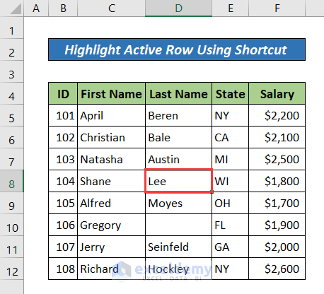
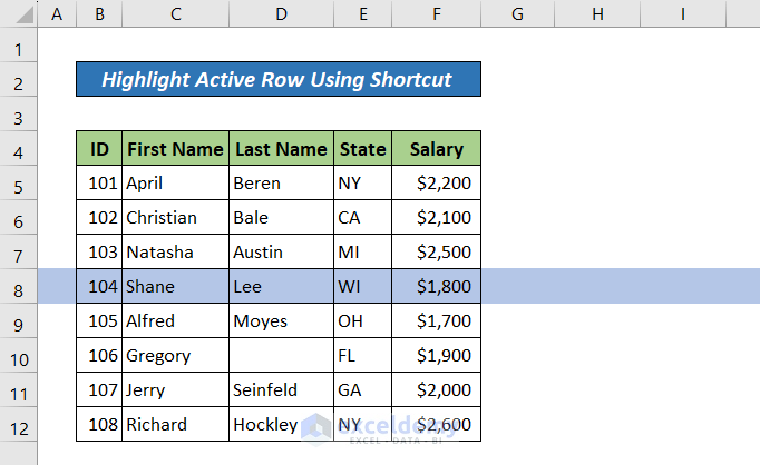
- Press Shift + Spacebar together, and the active row will be selected.
- From the Fill color option in the Font ribbon.
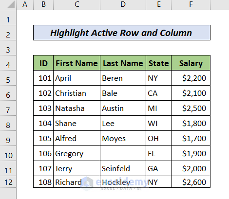
Highlight Active Row and Column at Once
- Apply VBA code to highlight active rows and columns in the following dataset.
- Right-click on the sheet name and select View Code.
- Insert the below-mentioned VBA code in the module.
Private Sub Worksheet_SelectionChange(ByVal SelectedRange As Range)

  If SelectedRange.Cells.Count > 1 Then Exit Sub

  Application.ScreenUpdating = False

  ' Clear the color of all cells

  Cells.Interior.Color = RGB(255, 255, 255) ' White color

  With SelectedRange

    ' Highlight row and column of the selected cell

    .EntireRow.Interior.Color = RGB(200, 200, 200) ' Light gray color

    .EntireColumn.Interior.Color = RGB(0, 255, 255) ' Cyan color

  End With

  Application.ScreenUpdating = True

End Sub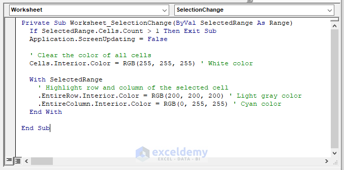
Code Breakdown
- If SelectedRange.Cells.Count > 1 Then Exit Sub: If the selected range exceeds 1, it will exit the sub. It will execute the remaining code.
- Cells.Interior.Color = RGB(255, 255, 255) ‘ White color: This line makes the cell background white.
- .EntireRow.Interior.Color = RGB(200, 200, 200) ‘ Light gray color: This line makes the entire row background color light gray.
- .EntireColumn.Interior.Color = RGB(0, 255, 255) ‘ Cyan color: This line makes the entire column background color Cyan.
- You will see that it will highlight both the row and the column of the active cell.

Things to Remember
- Check if any of your rows contains merged cells. Unmerge the cells before highlighting rows. Otherwise, it may not work as expected.
- If you have frozen panes in your Excel sheet, then the frozen row might not be highlighted if you select a row below the frozen pane. Adjust the frozen panes as needed or select a row within the unfrozen area.
Frequently Asked Questions
1. Can I remove the highlighting from a row in Excel?
Yes, you can remove the highlighting from a row in Excel. To do this, select the highlighted row, go to the “Home” tab, click on the “Fill Color” button, and choose “No Fill” or “Default” to remove the highlighting.
2. How can I quickly highlight alternating rows in Excel?
To quickly highlight alternating rows in Excel, you can use conditional formatting. In the “Conditional Formatting” button, choose “New Rule,” select the option “Use a formula to determine which cells to format,” and enter the formula “=MOD(ROW(),2)=0” for one formatting rule and “=MOD(ROW(),2)=1” for the other.
3. Does highlighting a row affect the data or formulas in Excel?
No, highlighting a row in Excel does not affect the underlying data or formulas.
Download Practice Workbook
Download the following Excel file for your practice.
How to Highlight a Row in Excel: Knowledge Hub
- Highlight Entire Row in Excel with Conditional Formatting
- Highlight Active Row
- Highlight Row If Cell Is Not Blank
- Highlight Row If Cell Contains Any Text
- Highlight Every 5 Rows
<< Go Back to Highlight in Excel | Learn Excel
Get FREE Advanced Excel Exercises with Solutions!
