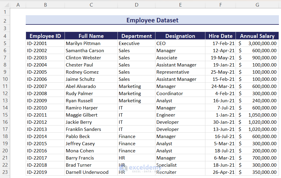
We have an Employee Dataset containing employee names, departments, designations, hiring dates, and annual salaries. In this dataset, we will highlight the rows depending on various conditions related to blank cells existing (or not existing) in rows or columns.
Read More: How to Highlight Row If Cell Contains Any Text in Excel
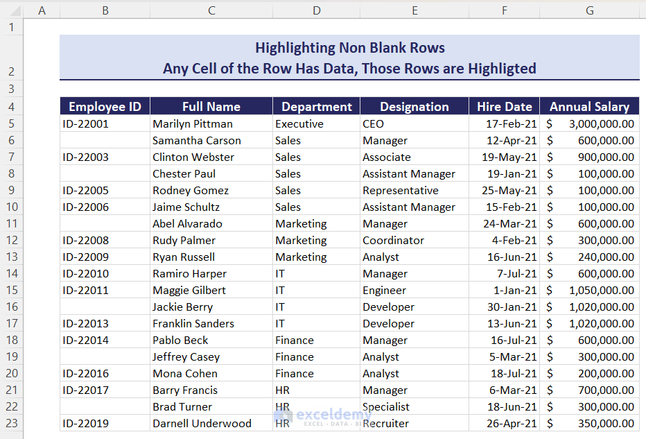
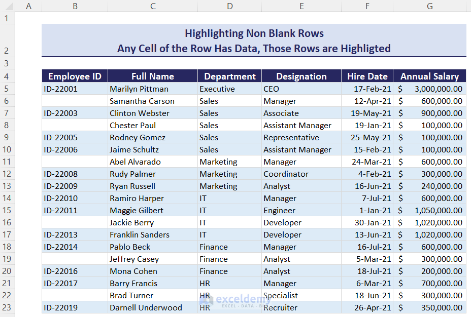
Method 1 – Highlighting a Row If the Row Contains No Blank Cells
We will highlight the rows where no cell is blank along the row, i.e. where every cell of the row has data.
Steps:
- Select the entire dataset (B5:G23 here) where you want to apply your conditional formatting.
- Go to the Home tab and choose the Conditional Formatting tool.
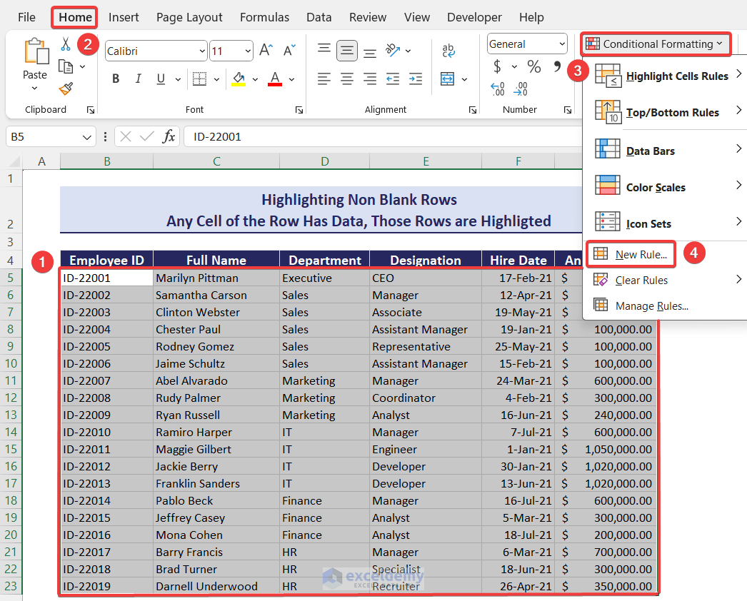
- Click on the New Rule… option. A New Formatting Rule window will appear.
- Choose the option Use a formula to determine which cells to format from the Select a Rule Type: options.
- Insert the following formula in the Format values where this formula is true: box.
=NOT(ISBLANK($B5))
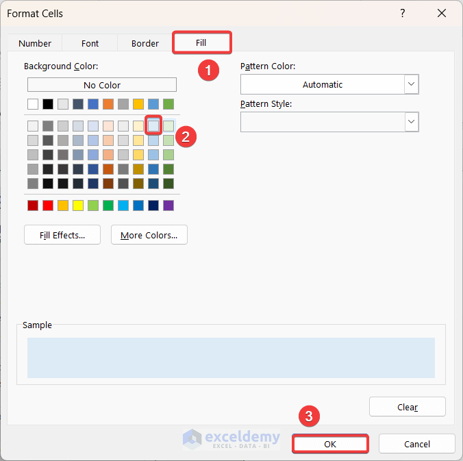
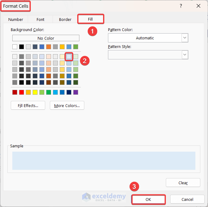
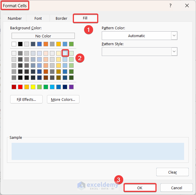
- Click the Format… button, and the Format Cells window will appear.
- Choose your desired highlighting format. We chose to fill the row with a light blue color.

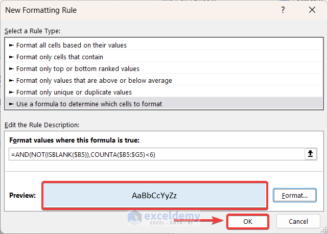
- Click on the OK button. The New Formatting Rule dialog box will appear again with a preview of the formatting.
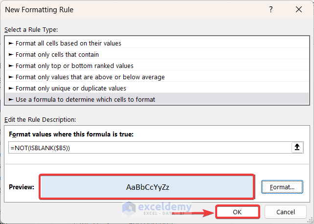
- Click on the OK button.
- You’ll get the result.
Read More: How to Highlight Every 5 Rows in Excel
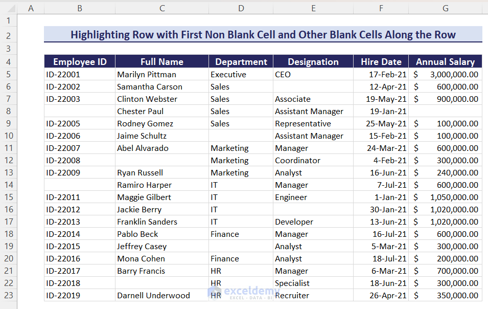
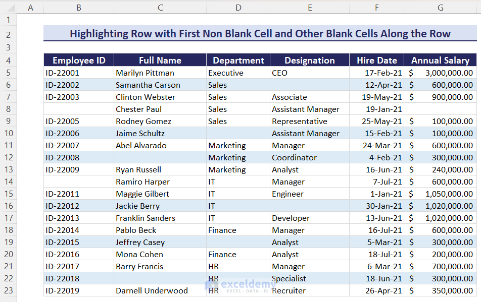
Method 2 – Highlighting a Row If the First Cell of the Row Is Not Blank but Some Other Cells Are Blank Along the Row
We will highlight rows that have data in the first column but contain blanks at some other cells along the row. But, if the first data is blank, then we will ignore the highlighting.
Steps:
- Select your dataset (cells B5:G23 here) where you want to highlight the rows.
- Click on the Home tab and go to Conditional Formatting.
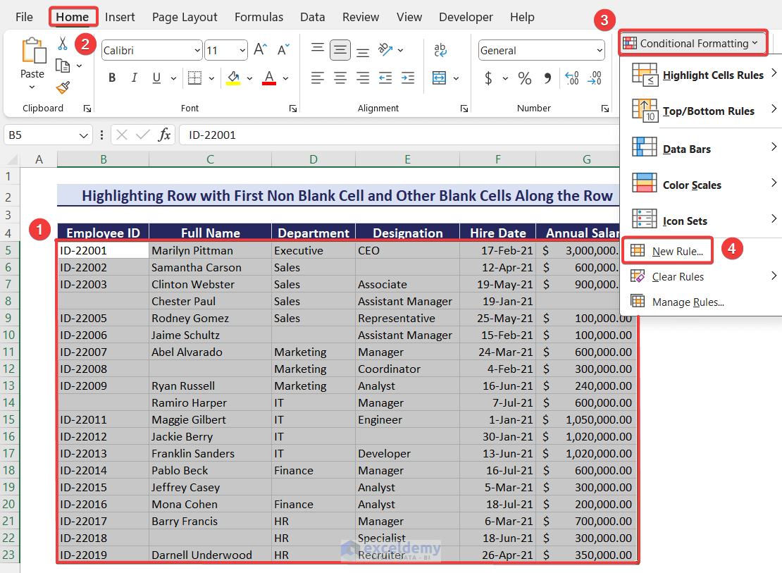
- Click on the New Rule… option to open the New Formatting Rule window.
- Choose the option Use a formula to determine which cells to format option from Select a Rule Type: options.
- Insert the following formula in the Format values where this formula is true: text box.
=AND(NOT(ISBLANK($B5)),COUNTA($B5:$G5)<6)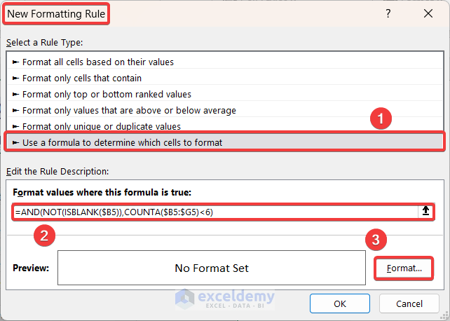
- Click the Format button.
- In the Format Cells window, select your preferred Fill color (or other formatting options) and click OK.
- You will find your finalized formatting with all selected options and chosen format displayed in the Preview: box.
- Click OK.
- Here’s the result.
Formula Breakdown:
=AND(NOT(ISBLANK($B5)),COUNTA($B5:$G5)<6)
=AND(NOT(ISBLANK($B5)),FALSE)// COUNTA($B5:$G5)<6 counts non-blank cells between cells B5:G5 and then compares the value if it is less than 6.
=AND(TRUE,FALSE)// NOT(ISBLANK($B5)) checks if cell B5 is blank or not and returns TRUE if not blank.
= FALSE// AND(TRUE,FALSE) returns true if all parameters are true and FALSE if any parameter is false.
How to Highlight a Row If Any Cell of the Row Contains a Specific Value in Excel
Case 1 – The Cell Contains a Specific Text
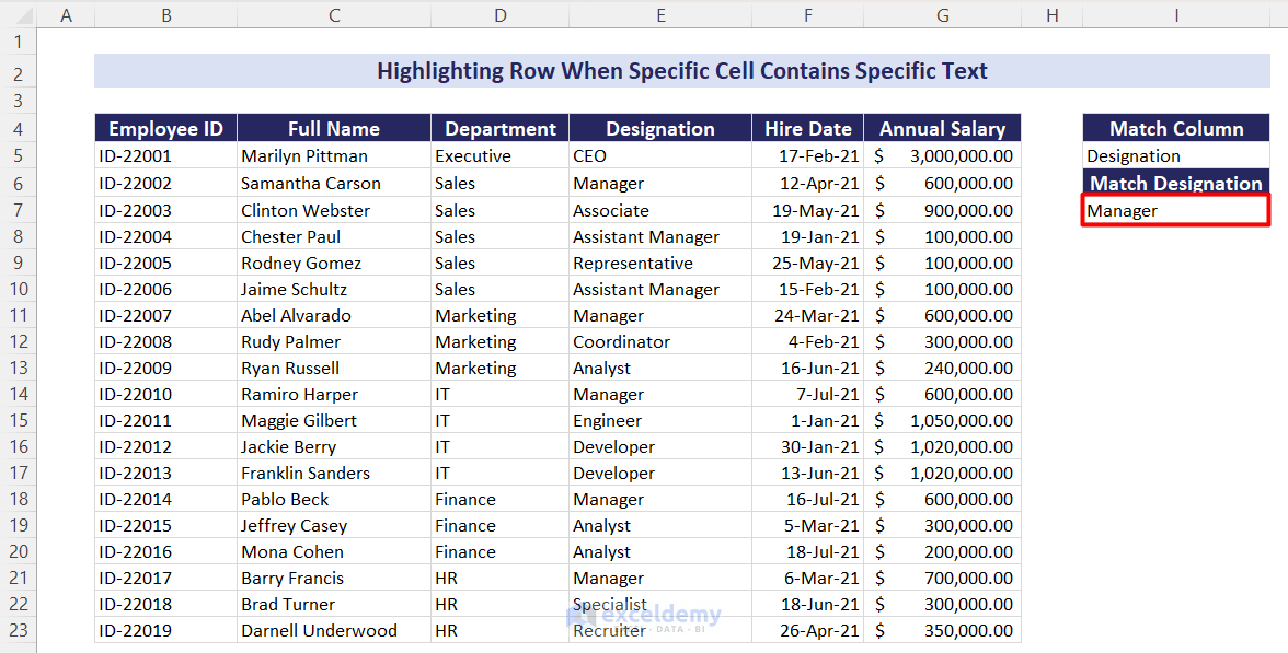
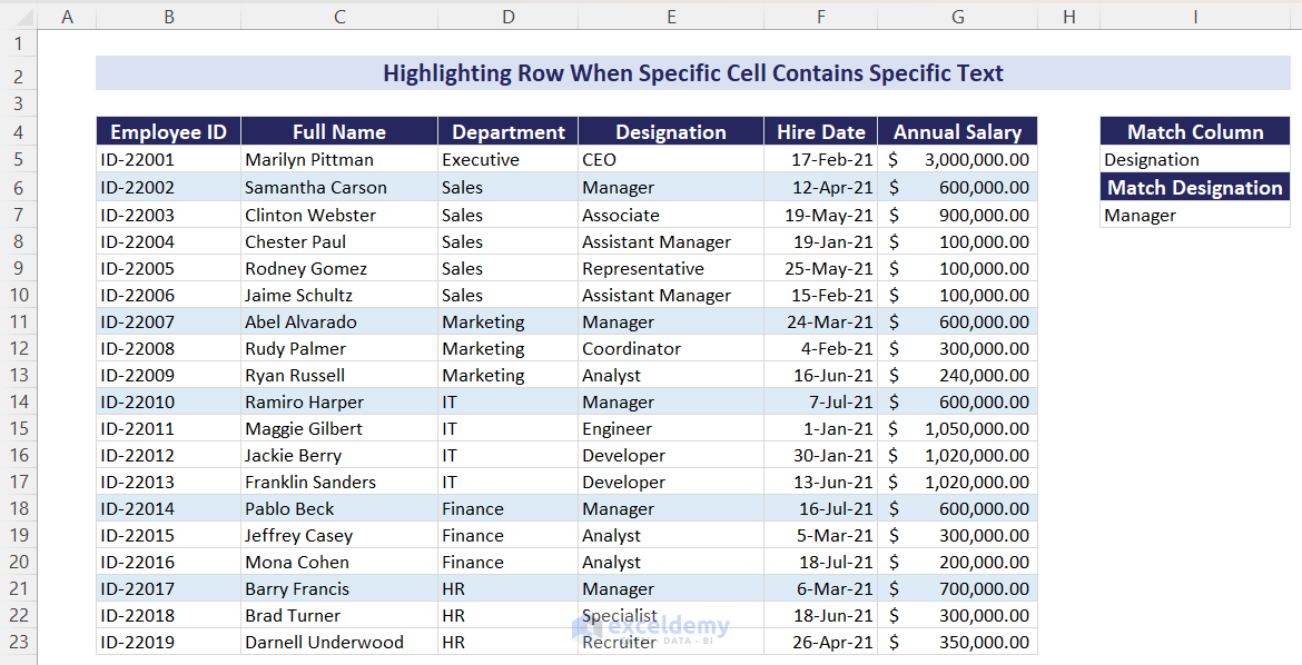
We’ll highlight the rows that contain a specific employee name, department, or designation based on a dynamic choice of selection by the user. We’ll create a dropdown list with Data Validation and then apply conditional formatting to highlight the desired rows.
Steps:
- Click on cell I5.
- Go to Data tab and select Data Validation.
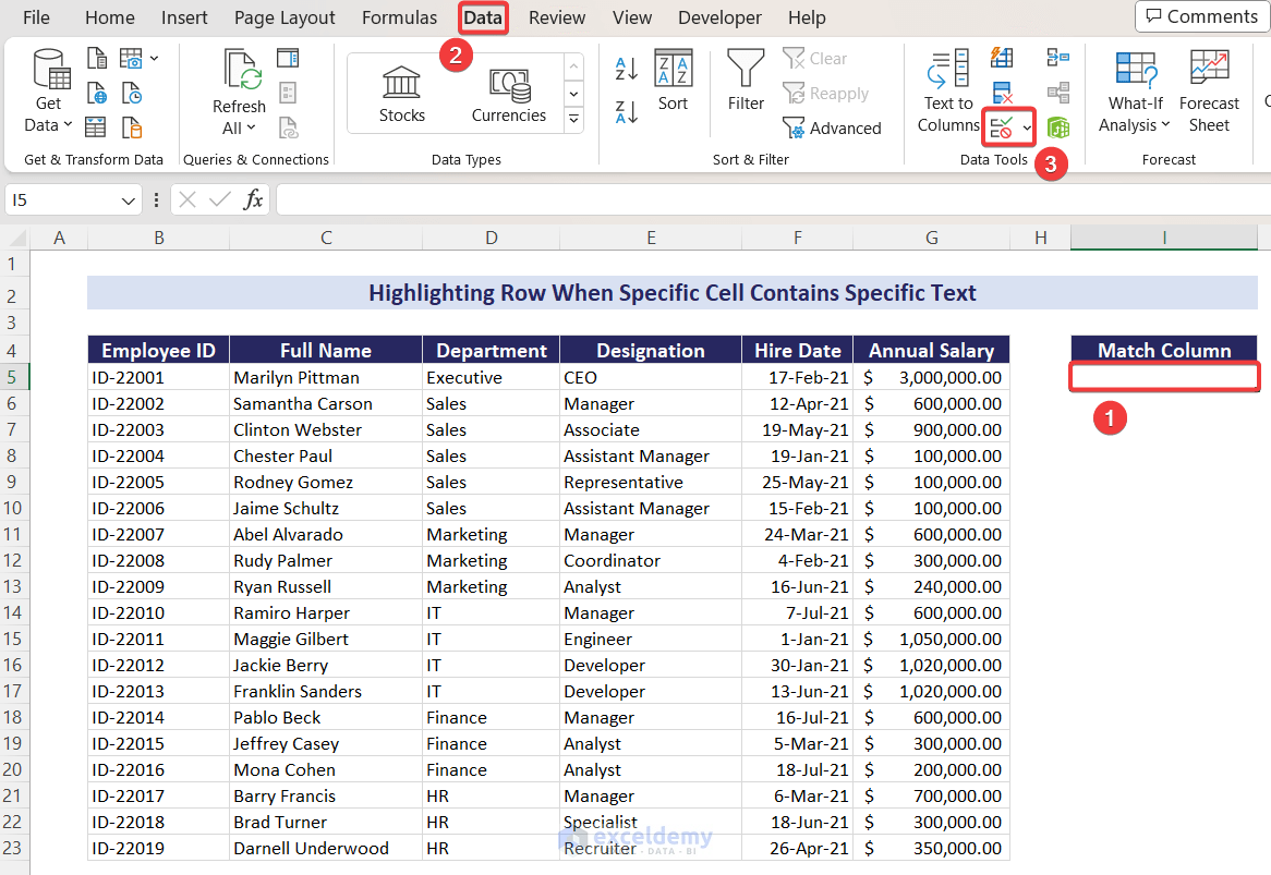
- The Data Validation window will appear. Choose the option List from Allow: dropdown options and reference cells C4:E4 in the Source: text box, as we want employee name, department, and designation in our dynamic list.
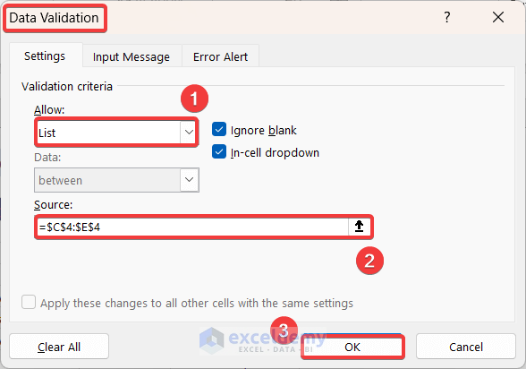
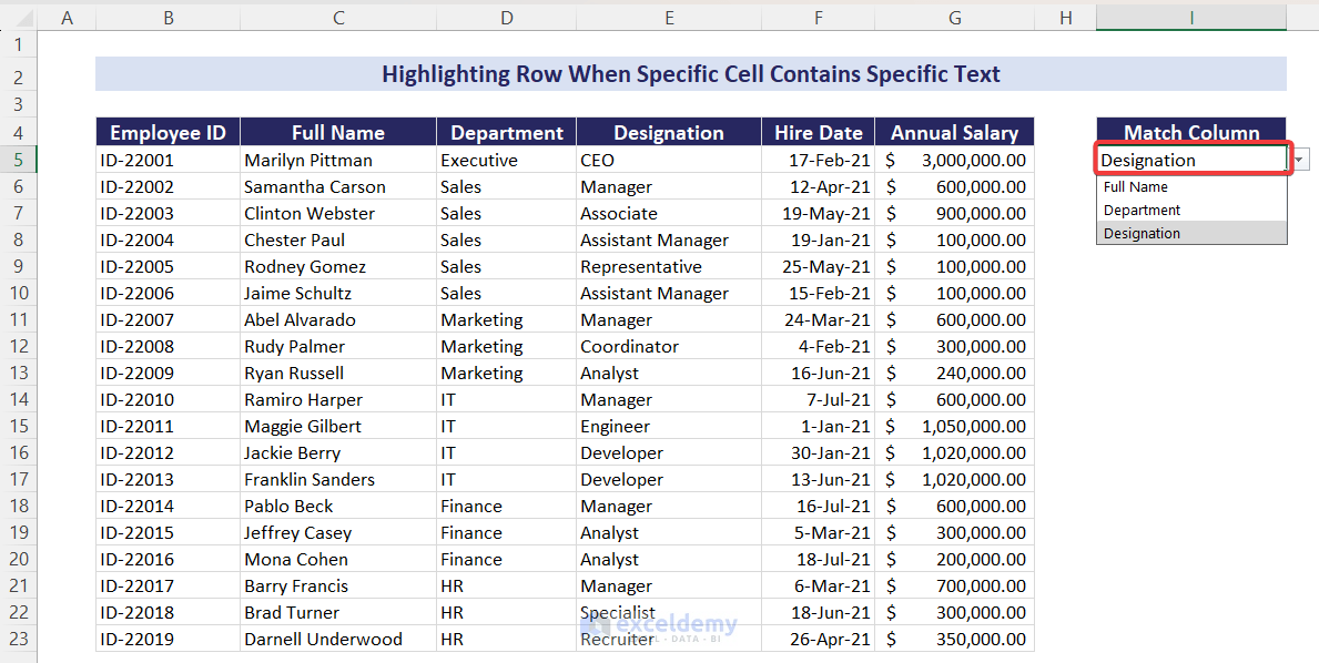
- Click on the OK button and you will get your desired dropdown list containing Full Name, Department, and Designation options.
- Choose any option that you want as a criterion to match to highlight rows.
- Click on cell I6 and insert the following formula:
="Match "&$I$5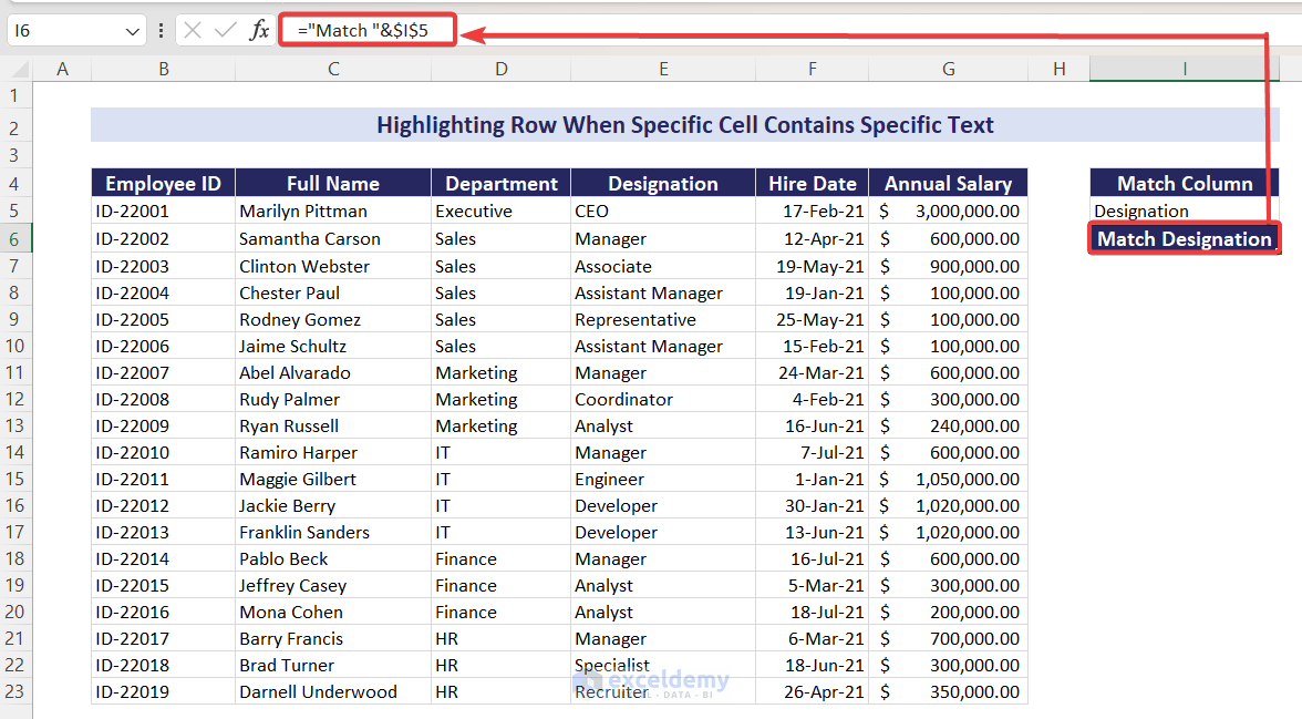
- Put the value you want to match in I7. Let’s say we want to match for Manager.
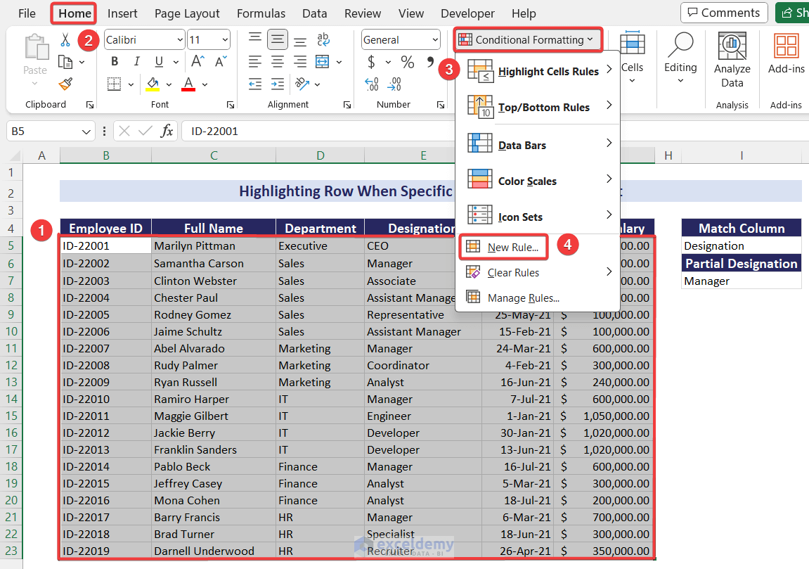
- Select the entire dataset.
- Go to Conditional Formatting and select New Rule…
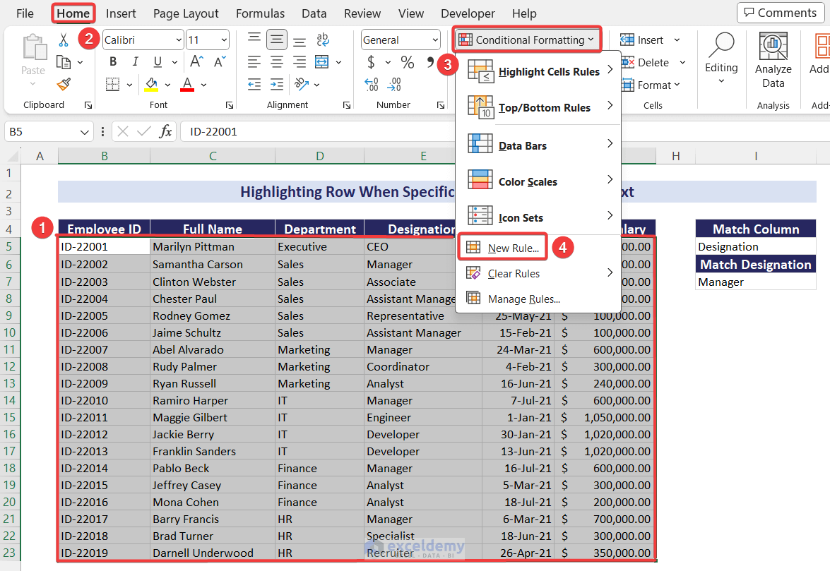
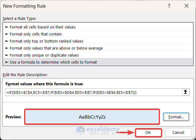
- The New Formatting Rule window will appear. Choose the Use a formula to determine which cells to format option from Select a Rule Type: and enter the following formula in the Format values where this formula is true: text box.
=IF($I$5=$C$4,$C5=$I$7,IF($I$5=$D$4,$D5=$I$7,IF($I$5=$E$4,$E5=$I$7)))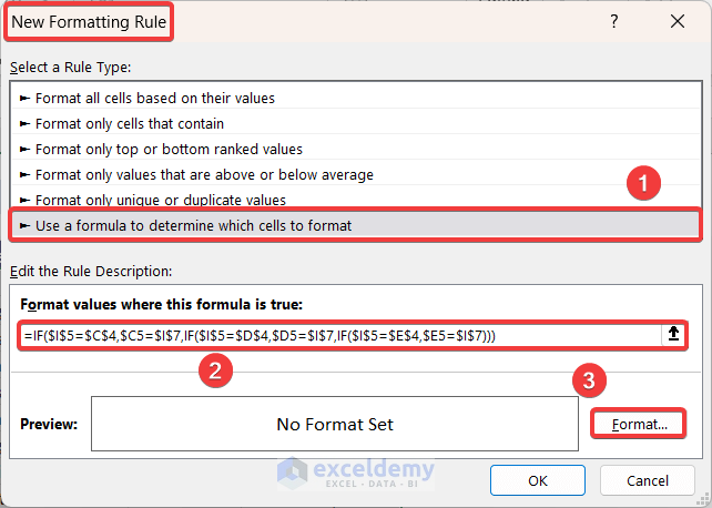
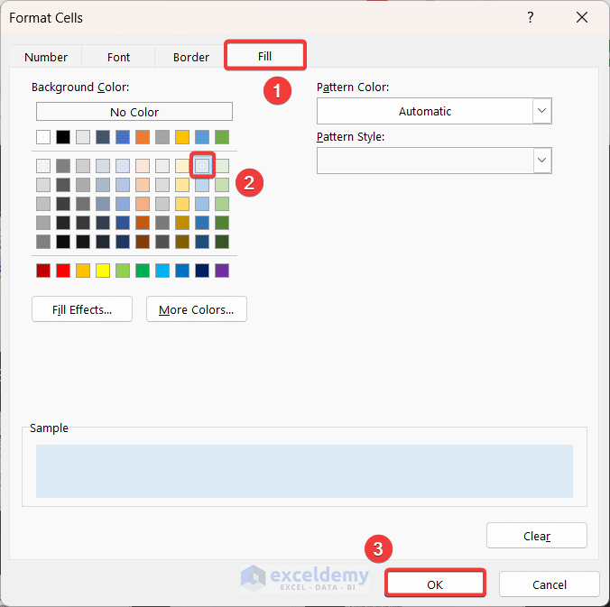
- To apply your desired formatting, click on the Format… button. Choose a Fill color and apply other styles as needed.
- Click OK.
- You’ll get the formatting preview shown in the Preview: box.
- Click on OK.
- We’ll get all the rows highlighted that contain Manager as the Designation value.
- You can select other dropdown options and input other values as well to highlight those rows.
Formula Breakdown:
=IF($I$5=$C$4,$C5=$I$7,IF($I$5=$D$4,$D5=$I$7,IF($I$5=$E$4,$E5=$I$7)))
=IF($I$5=$C$4,$C5=$I$7,IF($I$5=$D$4,$D5=$I$7,IF($I$5=$E$4,$E5=$I$7))) // IF($I$5=$E$4,$E5=$I$7) checks if cell I5 (Designation) matches cell E4 (Designation). If it is True, then it checks if cell E5 (CEO) matches cell I7 (Manager). Otherwise, it returns False.
=IF($I$5=$C$4,$C5=$I$7,IF($I$5=$D$4,$D5=$I$7,False)) // IF($I$5=$D$4,$D5=$I$7) checks if cell I5 (Designation) matches cell D4 (Department). If it matches then it checks if cell D5 (Executive) matches cell I7 (Manager).
=IF($I$5=$C$4,$C5=$I$7,False,False)) // IF($I$5=$C$4,$C5=$I$7) checks if cell I5 (Designation) matches cell C4 (Full Name). If it matches, then it checks if cell C5 (Marilyn Pittman) matches cell I7 (Manager). Otherwise, it returns False.
=False
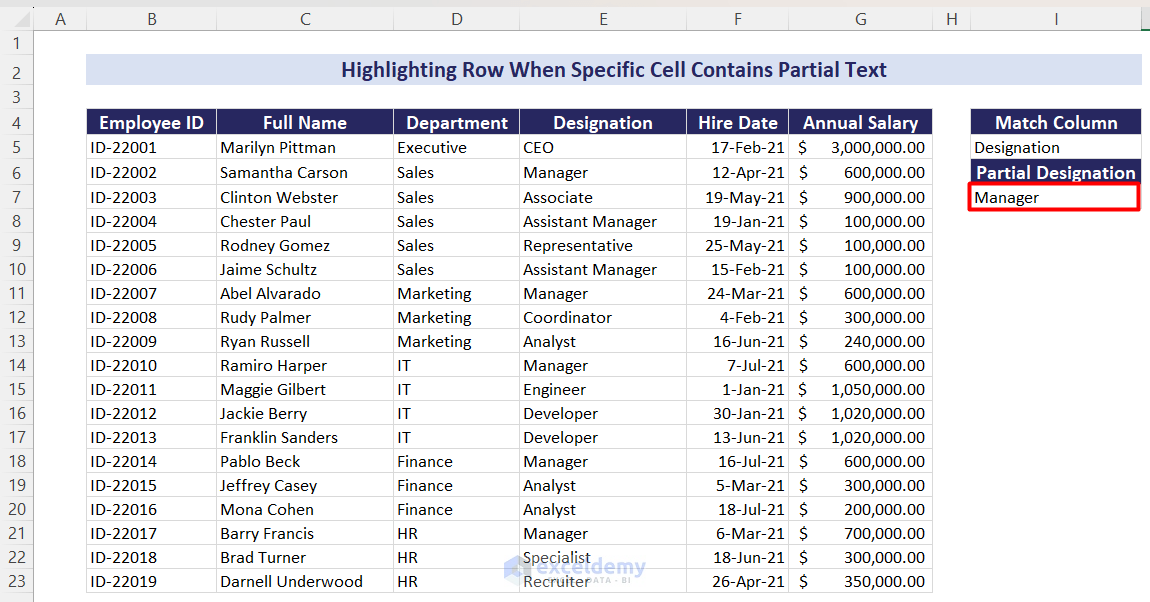
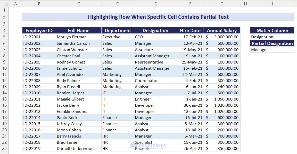
Case 2 – Cell Contains Specific Partial Text
In our dataset, we can see that we have designations as both Manager and Assistant Manager. We want to highlight rows that contain either of these designations.
Steps:
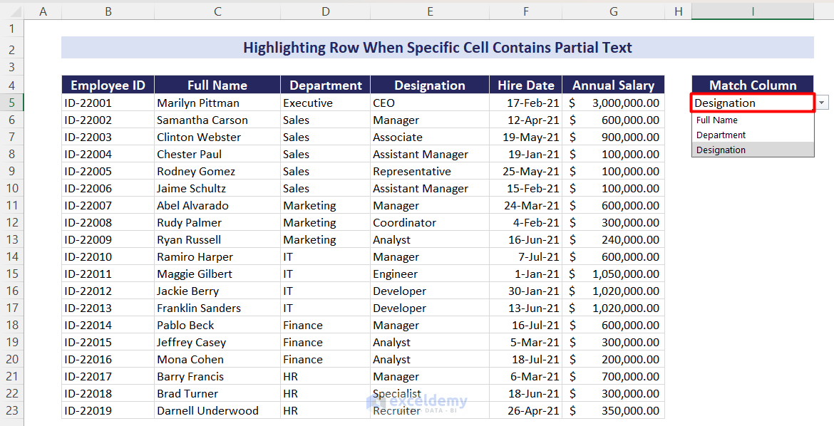
- Create a dropdown list like the previous case to set available criteria options such as Full Name, Department, and Designation.
- To show the partially matched column heading, insert the following formula in cell I6:.
="Partial "&$I$5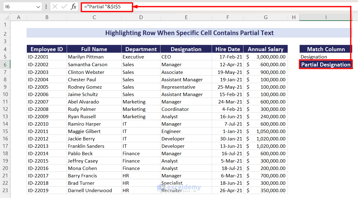
- Insert your desired partial match input in cell I7.
- Insert a new conditional formatting rule to the entire dataset.
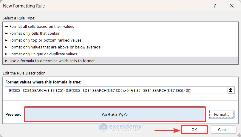
- The New Formatting Rule window appears. Choose the option Use a formula to determine which cells to format from Select a Rule Type: options.
- Insert the formula below in Format values where this formula is true: text box.
=IF($I$5=$C$4,SEARCH($I$7,$C5)>0,IF($I$5=$D$4,SEARCH($I$7,$D5)>0,IF($I$5=$E$4,SEARCH($I$7,$E5)>0)))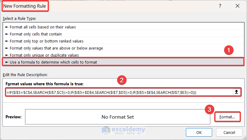
- Click on the Format… button to apply your desired format, then click OK to leave the section.
- Click on the OK button to finalize your New Formatting Rule window.
- You will find that all the rows with partially matched Manager designations are highlighted.
Formula Breakdown:
=IF($I$5=$C$4,SEARCH($I$7,$C5)>0,IF($I$5=$D$4,SEARCH($I$7,$D5)>0,IF($I$5=$E$4,SEARCH($I$7,$E5)>0)))
=IF($I$5=$C$4,SEARCH($I$7,$C5)>0,IF($I$5=$D$4,SEARCH($I$7,$D5)>0,IF($I$5=$E$4,SEARCH($I$7,$E5)>0))) // IF($I$5=$E$4,SEARCH($I$7,$E5)>0) checks if cell I5 (Designation) matches cell E4 (Designation). If it is a match, then it will search cell I7 (Manager) appearances in cell E5 (CEO) and will count if this search result appears greater than zero times.
=IF($I$5=$C$4,SEARCH($I$7,$C5)>0,IF($I$5=$D$4,SEARCH($I$7,$D5)>0,False)) // IF($I$5=$D$4,SEARCH($I$7,$D5)>0 checks if cell I5 (Designation) matches cell D4 (Department). If it is a match, then it will search cell I7 (Manager) appearances in cell D5 (Executive) and will count if this search result appears greater than zero times.
=IF($I$5=$C$4,SEARCH($I$7,$C5)>0,False,False)) // IF($I$5=$C$4,SEARCH($I$7,$C5)>0) checks if cell I5 (Designation) matches cell C4 (Full Name). If it is a match, then it will search cell I7 (Manager) in cell C5 (Marilyn Pitman) and will count if this search result appears greater than zero times.
=FALSE
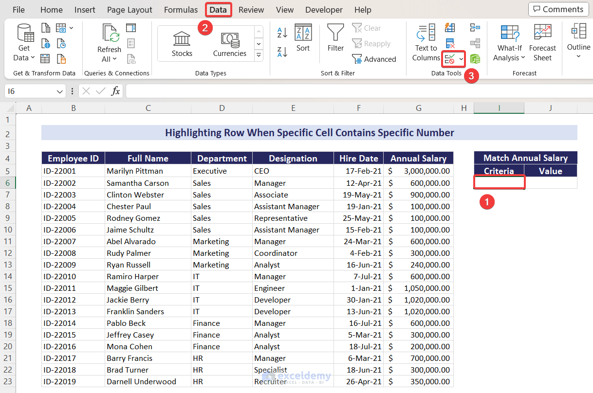
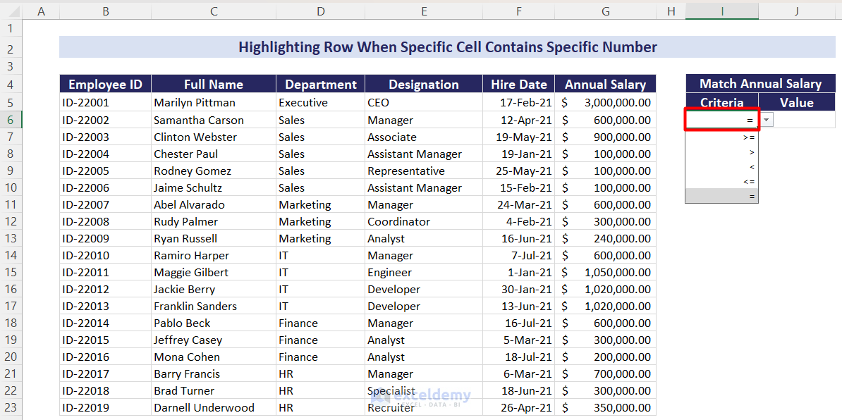
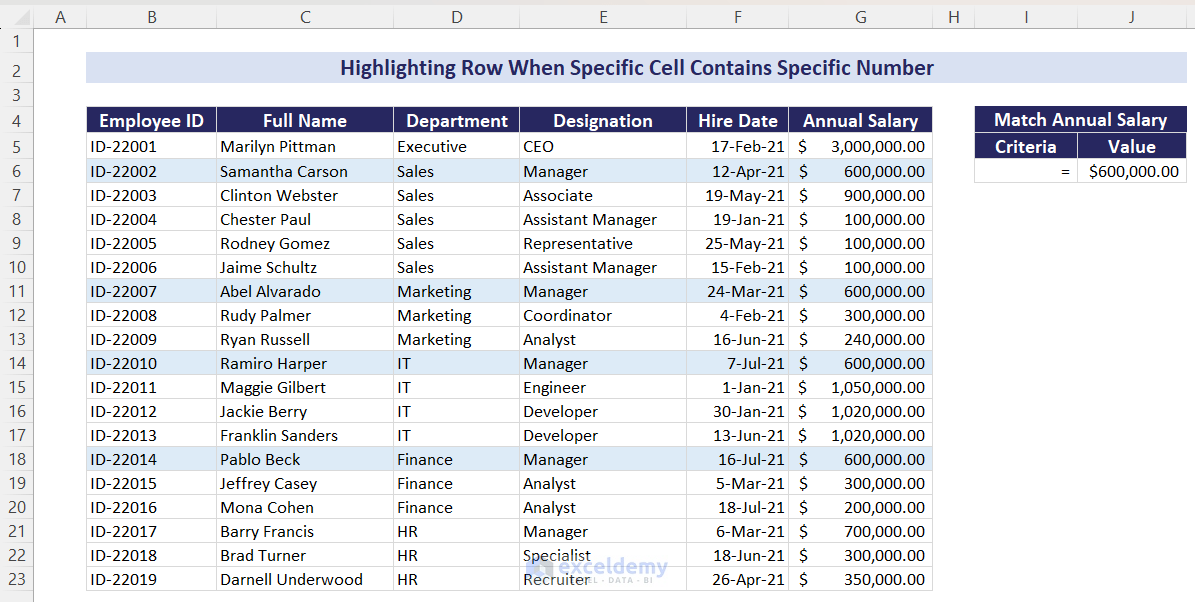
Case 3 – A Specific Cell Contains a Specific Number
We will highlight rows that contain specific salaries or a specific range of salaries.
Steps:
- Select cell I6 and go to Data tab.
- Choose the Data Validation tool.
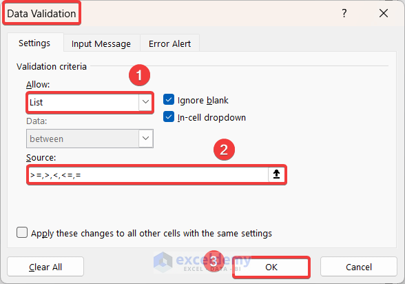
- The Data Validation window appears. Choose List in Allow: dropdown options.
- Insert the following symbols with separated commas (>=, >, <, <=, =) in the Source: text box.
- Click on OK and the data validation is active.
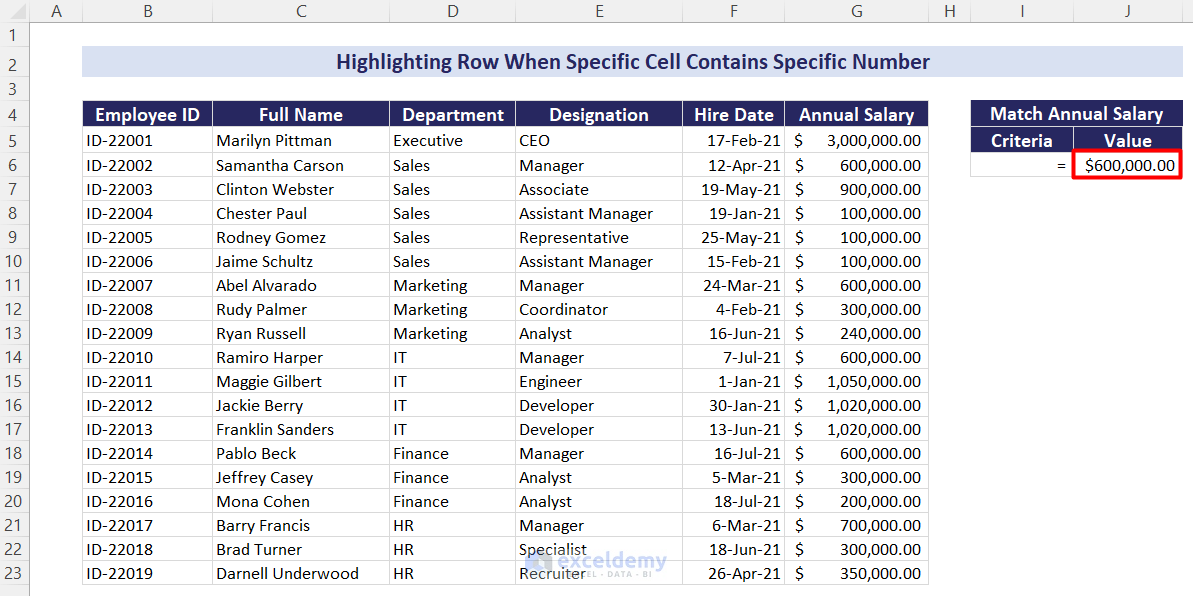
- Choose your desired criteria (= for our example) operator from the dropdown.
- Insert your desired specific value in cell J6 (600000 here).
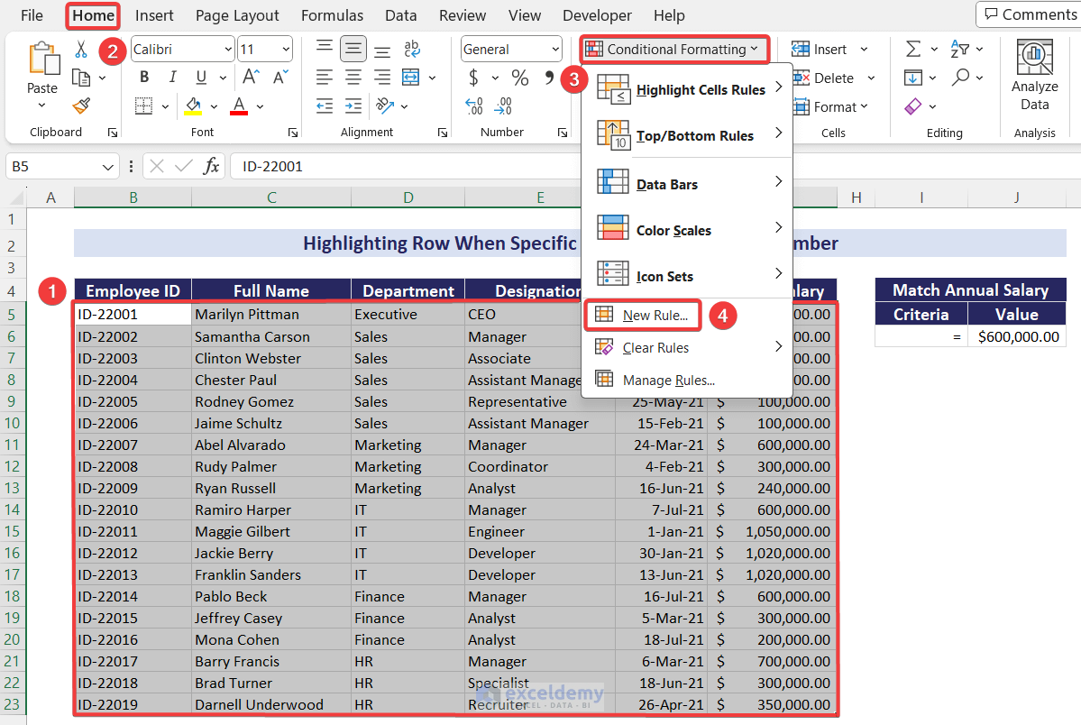
- To apply conditional formatting, select your dataset and go to Conditional Formatting, then select New Rule…
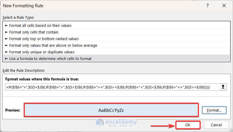
- Choose the option Use a formula to determine which cells to format from Select a Rule Type: and insert the following formula in the Format values where this formula is true: text box.
=IF($I$6="=",$G5=$J$6,IF($I$6=">",$G5>$J$6,IF($I$6=">=",$G5>=$J$6,IF($I$6="<",$G5<$J$6,IF($I$6="<=",$G5<=$J$6)))))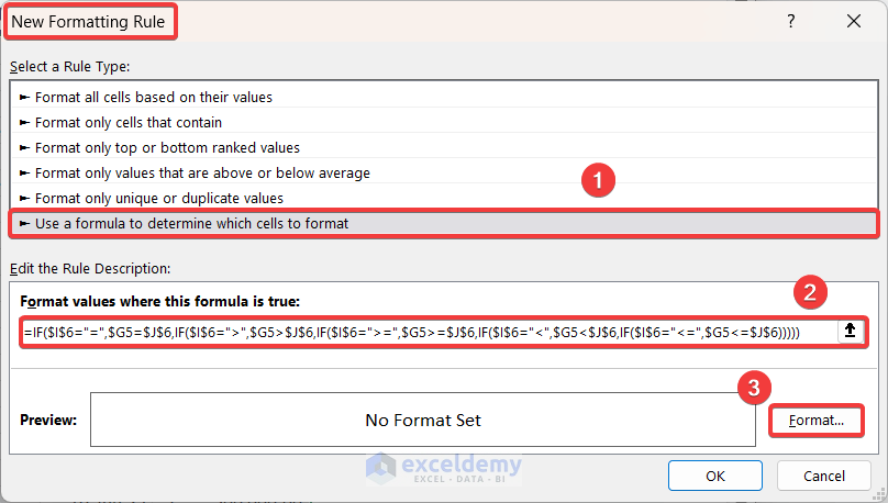
- Click on the Format… button. Choose your highlighting format as your wish.
- Click OK.
- Here’s the preview.
- Click OK.
- Here are the results of the sample we used.
- You can select any other criteria from the dropdown and insert any other value to highlight rows according to your own target.
Formula Breakdown:
=IF($I$6=”=”,$G5=$J$6,IF($I$6=”>”,$G5>$J$6,IF($I$6=”>=”,$G5>=$J$6,IF($I$6=”<“,$G5<$J$6,IF($I$6=”<=”,$G5<=$J$6)))))
=IF($I$6=”=”,$G5=$J$6,IF($I$6=”>”,$G5>$J$6,IF($I$6=”>=”,$G5>=$J$6,IF($I$6=”<“,$G5<$J$6,IF($I$6=”<=”,$G5<=$J$6))))) // IF($I$6=”<=”,$G5<=$J$6) checks if cell I6 (=) contains “<=” operator. If it is True, then it checks if cell G5 (3,000,000) is less than or equal to cell J6 (600,000).
=IF($I$6=”=”,$G5=$J$6,IF($I$6=”>”,$G5>$J$6,IF($I$6=”>=”,$G5>=$J$6,IF($I$6=”<“,$G5<$J$6,False)))) // IF($I$6=”<“,$G5<$J$6) checks if cell I6(=) contains “<” operator. If it is True, then it compares if cell G5 (3,000,000) is less than cell J6 (600,000).
=IF($I$6=”=”,$G5=$J$6,IF($I$6=”>”,$G5>$J$6,IF($I$6=”>=”,$G5>=$J$6,False,False)))) // IF($I$6=”>=”,$G5>=$J$6) checks if cell I6 (=) contains “>=” operator. If it is True, then it checks if cell G5 (3,000,000) is greater than or equal to cell J6 (600,000).
=IF($I$6=”=”,$G5=$J$6,IF($I$6=”>”,$G5>$J$6,False,False,False)))) // IF($I$6=”>”,$G5>$J$6) checks if cell I6 (=) contains “>” operator. If it is True, then it checks if cell G5 (3,000,000) is greater than cell J6 (600,000).
=IF($I$6=”=”,$G5=$J$6,False,False,False,False)))) // IF($I$6=”=”,$G5=$J$6) checks if cell I6 (=) contains “=” operator. If it is True, then it checks if cell G5 (3,000,000) is equal to cell J6 (600,000).
= FALSE
Download the Practice Workbook
Related Articles
- How to Highlight Entire Row in Excel with Conditional Formatting
- How to Highlight Active Row in Excel
<< Go Back to Highlight Row | Highlight in Excel | Learn Excel
Get FREE Advanced Excel Exercises with Solutions!

How to highlight the enter row if all cells in selection of that row are blank?
Thanks a lot for your question. Here, if all of the cells on a single row are blank in your dataset, they will be highlighted if you follow this tutorial. If you have any further issues, feel free to inform us again.
Each time you used the word “Row” you really meant “Cell”. Your title suggests you would show how to highlight the ENTIRE Row if a specific cell was blank. Can you do that?
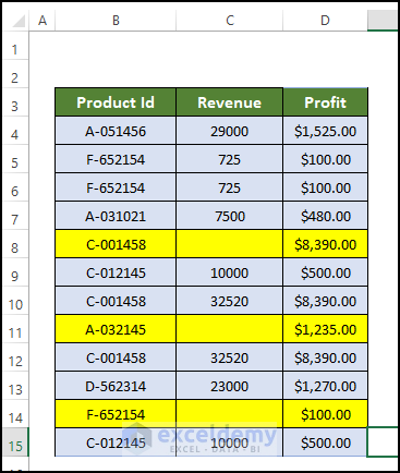
Thanks a lot for your question, Aaron. Here we are going to use a separate formula for highlighting the entire row based on whether any of the values in the row are blank or not. Notice the image below, we got blank cell in C8,C11, and C14
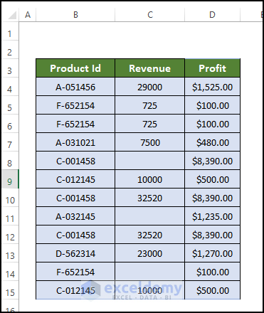
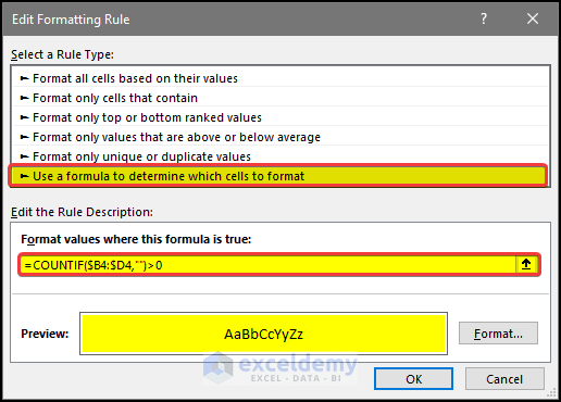
2. First, go to the Conditional Formatting, and set the rules as shown below.
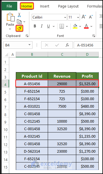
3. Then select only the B4:D4, and copy the formatting style of this cell.
4. Paste the formatting style all over the range of B4:D15.
And now you can see that the rows now highlighted if there is any blank cell in the entire row.
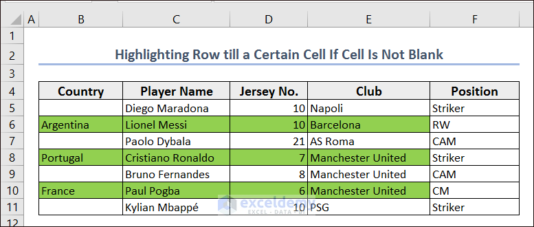
Is there a way to format a row until a point, instead of the entire row? For example, if you typed something into column B, the same formatting rule would be applied to columns B through J in that row (stopping at J), instead of the entirety of the row. Method 1 would be perfect for my needs if the conditional formatting rule didn’t continue onwards into infinity. Or is that too complicated for Excel to do?
Hello JAKE,
Thanks for your response.
The simplest way to highlight rows till a specific cell, instead of the entire row is to select the range till that column before applying the conditional formatting.
Then, you can apply any of the above methods and have your desired result.
If you have already applied the conditional formatting and want to change the selection range, go to the Home tab and click on Conditional Formatting. After that, select Manage Rules…
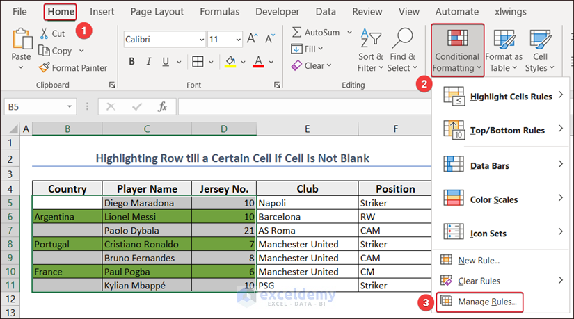
Now, change the range from the Applies to section and click on OK.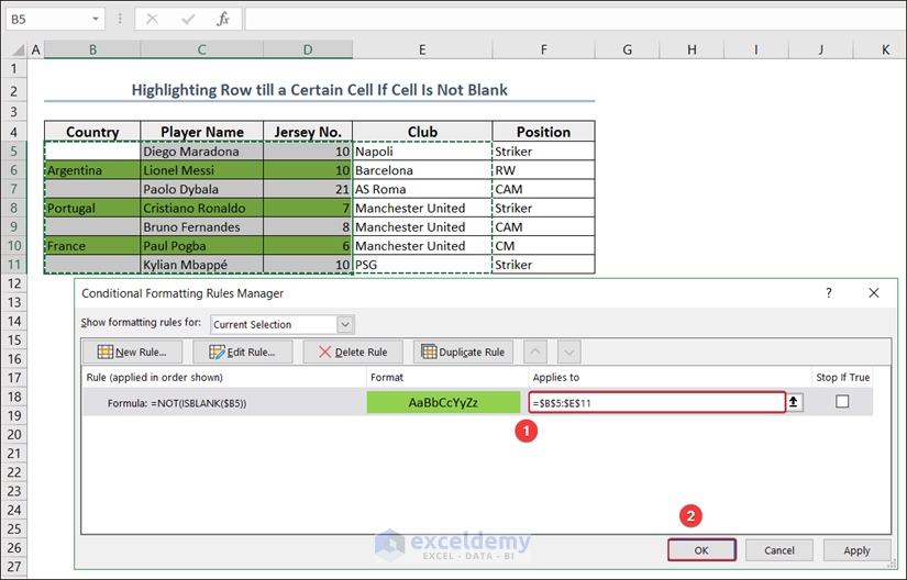
You will have the selection changed according to your desired cell.