How to Highlight Active Row in Excel (3 Methods)

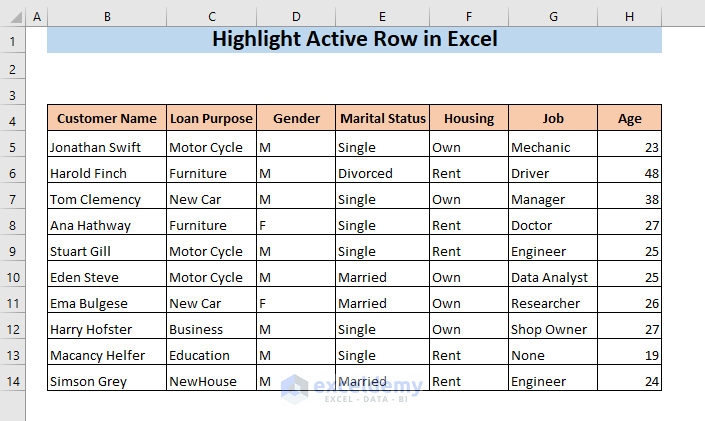
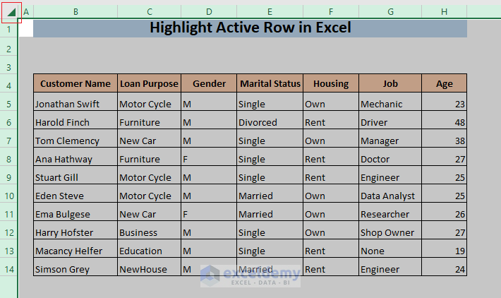
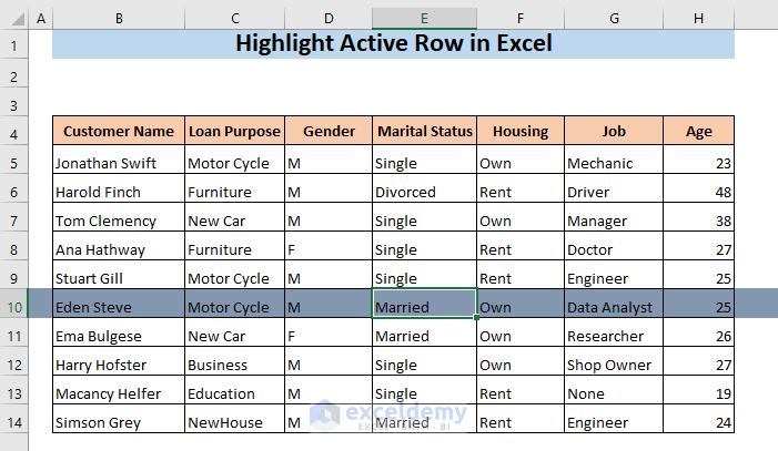
We’ll use the following sample dataset to highlight a row whenever we select a cell in that row.

Method 1 – Highlighting the Active Row by Using Conditional Formatting in Excel

• Select your entire worksheet by clicking on the top-left corner of the sheet.

• Go to Home, choose Conditional Formatting, and select New Rule.

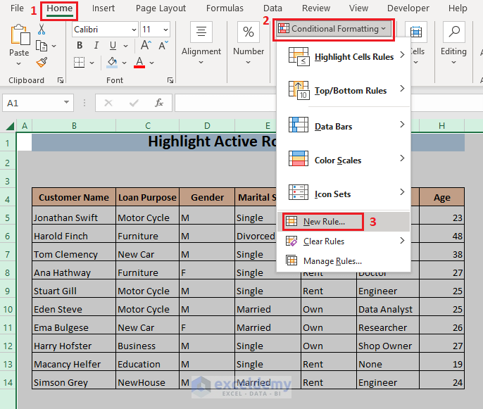
• This will open the New Formatting Rule window.
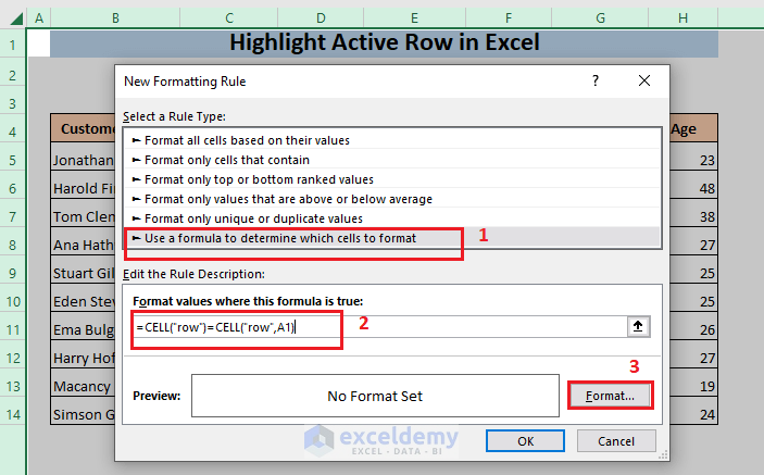
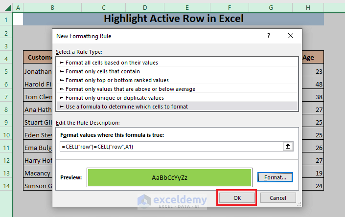
• Select Use a formula to determine which cells to format from Select a Rule Type.
• A new box named Format values where this formula is true will appear in the bottom part of the New Formatting Rule window.
• Use the following formula in the Format values where this formula is true box:

• Click on Format to set the color for highlighting.

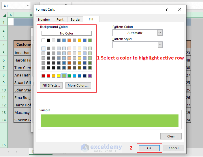
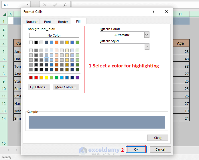
• A new window named Format Cells will appear.
• Select a color with which you want to highlight the active row from the Fill tab.
• You can also set different number formatting, font, and border styles for the active row in the other tabs of the Format Cells window if you want to.
• Click on OK.

• You will see your selected formatting style in the Preview box of the New Formatting Rule window.
• Click on OK.

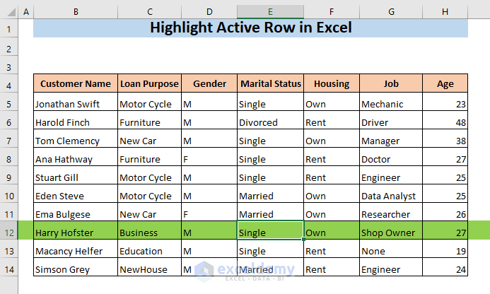
• Select any cell of your dataset.
• The entire row of the active cell will be highlighted with your selected color.

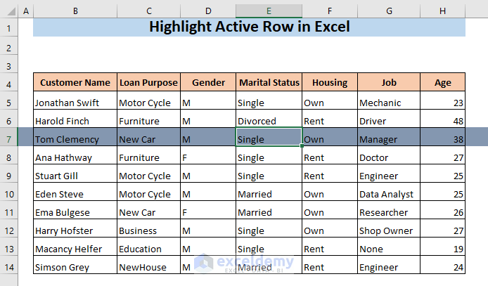
• If you select a cell from any other row, you will see the first row is still highlighted.

This is happening because Excel hasn’t refreshed itself. Excel automatically refreshes itself when a change is made in any cell or when a command is given. But it doesn’t refresh automatically when you just change your selection. So, you need to refresh Excel manually.

• Press F9.
• Select a cell and press F9 to highlight the active row and remove previous highlights.

Method 2 – Using VBA to Highlight Rows with Active Cell in Excel

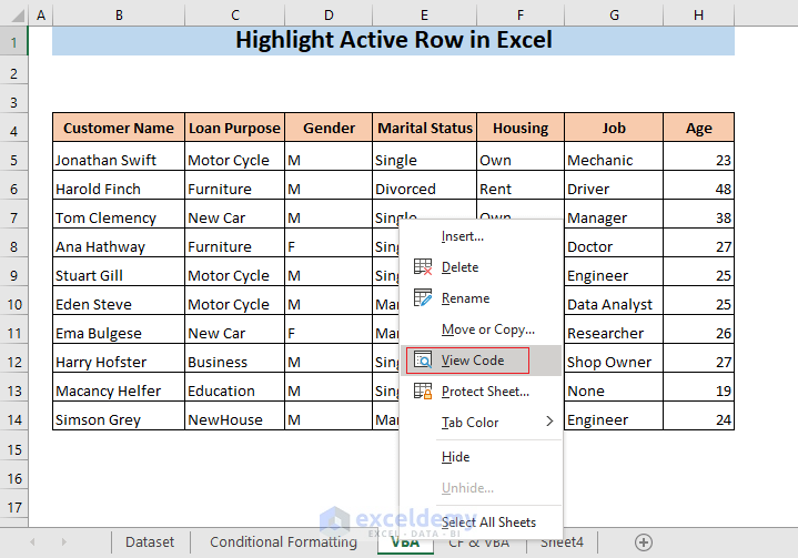
• Right-click on the sheet name (VBA) where you want to highlight the active row.
• Select View Code.

• This will open the VBA window. You will see the Code window of that sheet.

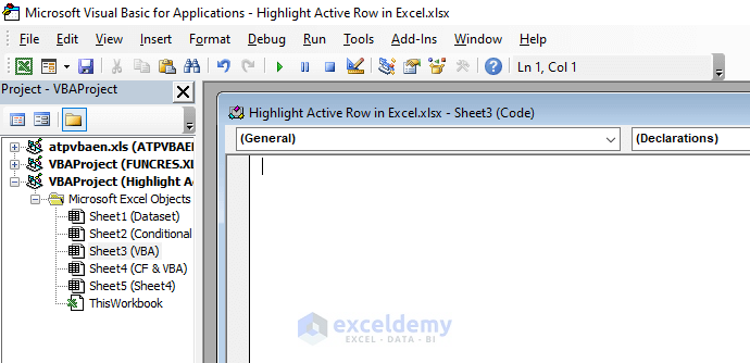
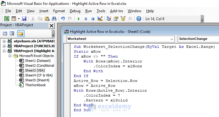
• Insert the following code in the window.

Sub Worksheet_SelectionChange(ByVal Target As Excel.Range)

Static xRow

If xRow <> "" Then
    With Rows(xRow).Interior
        .ColorIndex = xlNone
    End With
End If

Active_Row = Selection.Row
xRow = Active_Row
With Rows(Active_Row).Interior
    .ColorIndex = 7
    .Pattern = xlSolid
End With

End Sub

The code will change the color of the row with the selected cell with a color that has color index 7. If you want to highlight the active row with other colors, insert a number other than 7 in the .colorIndex value.

• Close or minimize the VBA window.
• If you select a cell, the whole row will be highlighted.

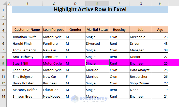
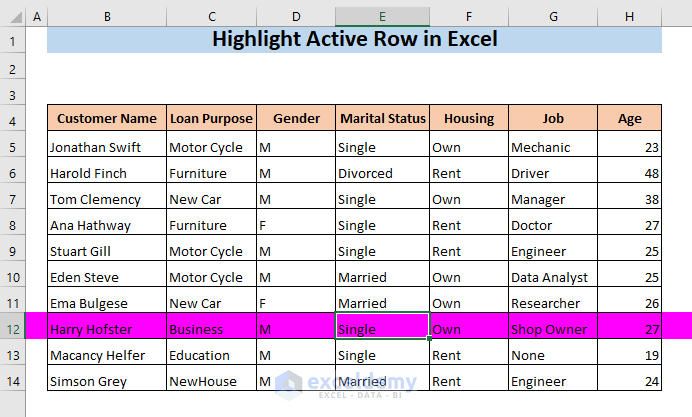
• Select another cell from a different row.
• The new row will be highlighted instead.

Read More: How to Highlight Entire Row in Excel with Conditional Formatting

Method 3 – Automatically Highlight the Active Row Using Conditional Formatting and VBA

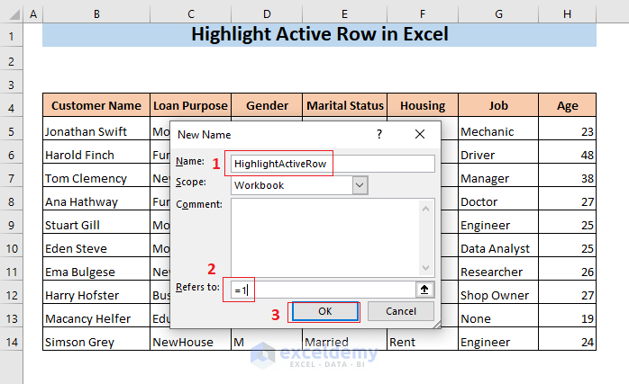
• Go to the Formulas tab and select Define Name.

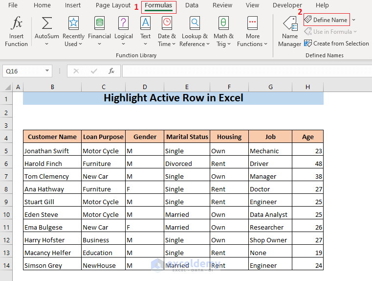
• This will open the New Name window.
• Type a name (for example HighlightActiveRow) in the Name box and put =1 in the Refers to box.
• Press OK.

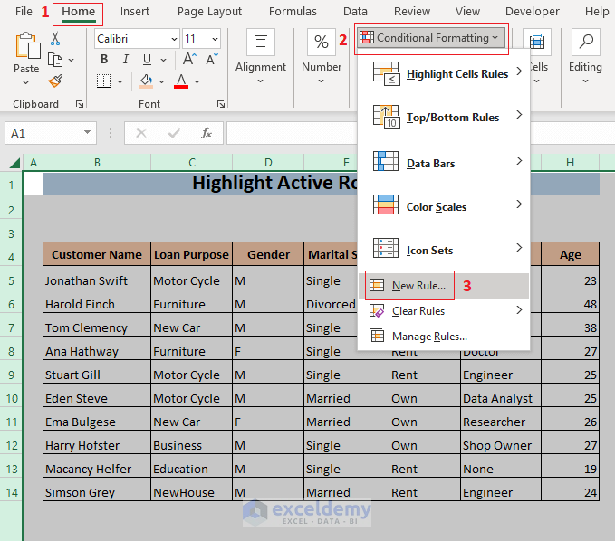
• Select the entire worksheet by clicking on the top-left corner of the sheet.

• Go to Home, then to Conditional Formatting, and select New Rule.

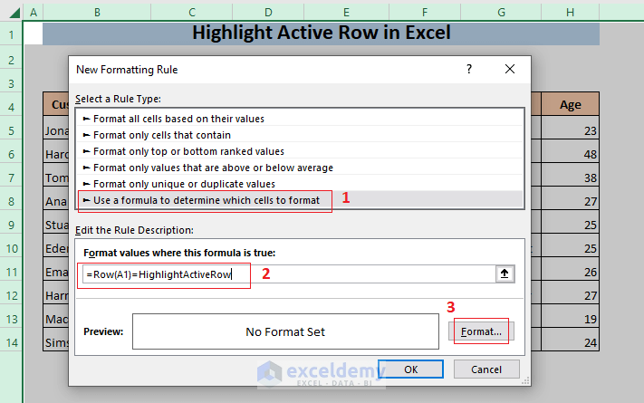
• This will open the New Formatting Rule window.
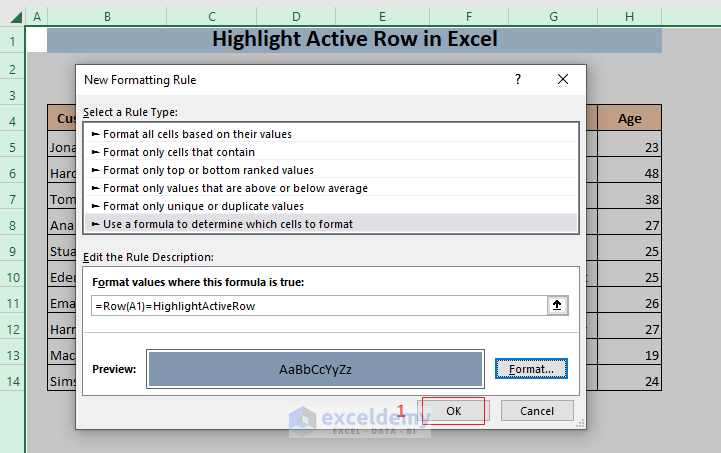
• Select Use a formula to determine which cells to format from the Select a Rule Type box.
• A new box named Format values where this formula is true will appear in the bottom part of the New Formatting Rule window.
• Use the following formula in the Format values where this formula is true box:

• Click on Format to set the color for highlighting.

• Select a color with which you want to highlight the active row from the Fill tab. You can also other formatting options by going to the different tabs of the Format Cells window.
• Click on OK.

• Click on OK again.

• Right-click on the sheet name (CF & VBA) where you want to highlight the active row.
• Select VIew Code.

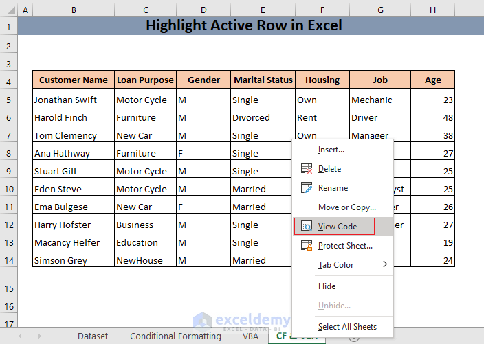
• Insert the following code in the VBA window that was opened.

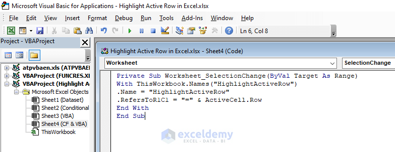
Private Sub Worksheet_SelectionChange(ByVal Target As Range)

    With ThisWorkbook.Names("HighlightActiveRow")
   .Name = "HighlightActiveRow"
   .RefersToR1C1 = "=" & ActiveCell.Row
    End With

End Sub

The code will automate the refreshing process. The name (HighlightActiveRow) must be the same as the name you have given in the Define Name box.

• Close or minimize the VBA window.
• If you select a cell, the whole row will be highlighted.

• If you select another cell, only the row of that cell will be highlighted.

Download the Practice Workbook

Related Articles

• How to Highlight Row If Cell Is Not Blank
• How to Highlight Row If Cell Contains Any Text in Excel
• How to Highlight Every 5 Rows in Excel
  

<< Go Back to Highlight Row | Highlight in Excel | Learn Excel