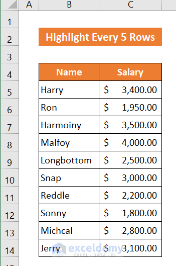
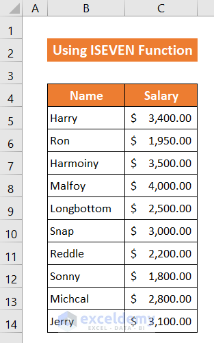
In this article, we will demonstrate how to highlight every 5 rows in an Excel workbook using 4 different methods. We’ll use the following dataset of 10 employees of a company and their salaries to illustrate our methods.
Method 1 – Using the ISEVEN, CEILING, and ROW Functions to Highlight Every 5 Rows
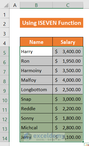
We can combine the ISEVEN, CEILING, and ROW functions to highlight every 5 rows. After completing the process, the last 5 rows will be filled in a different color.
Steps:
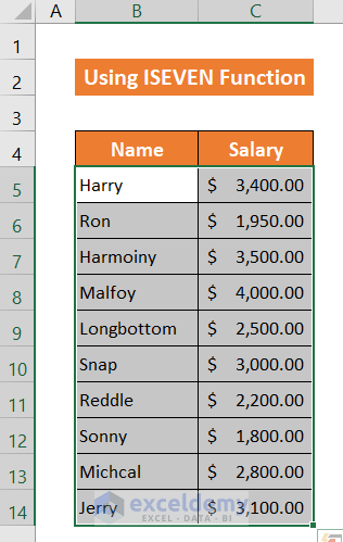
- Select the entire range B4:C14.
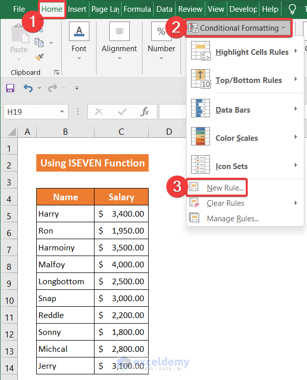
- In the Home tab, go to Conditional Formatting > New Rules.
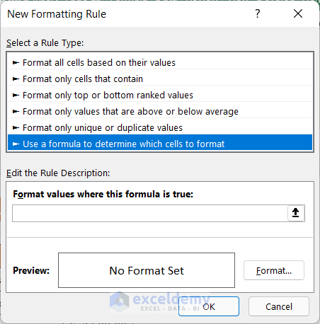
A new dialog box called New Formatting Rule will appear.
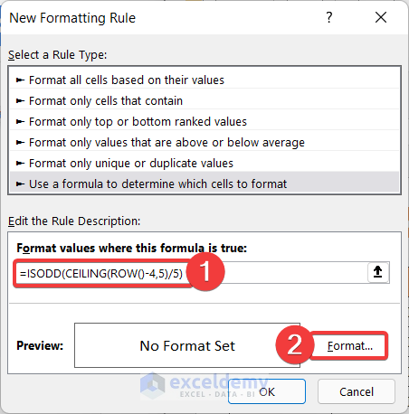
- Select Use a formula to determine which cells to format.
- Enter the following formula in the empty box:
=ISEVEN(CEILING(ROW()-4,5)/5)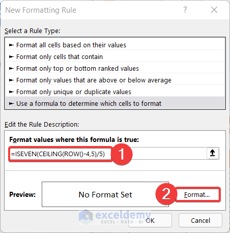
- Click Format.
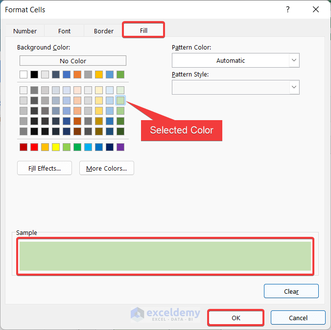
Another dialog box entitled Format Cells will appear.
- Go to the Fill tab.
By default the color of the cell will be white.
- Change the cell color, which will then appear in the Sample section. Here, we choose a light green color.
- Click OK to close the Format Cells dialog box.
- Click OK to close the New Formatting Rule box.
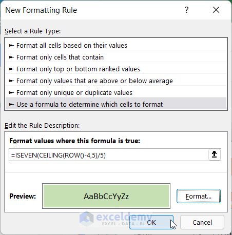
The last 5 rows of the list have our chosen highlight color.
Breakdown of the Formula
For Row 10:
ROW(): Returns 10.
CEILING(ROW()-4,5)/5): Returns 2.
ISEVEN(CEILING(ROW()-4,5)/5): Returns True, which means the value of the CEILING function is even, so the row will be highlighted.
Read More: How to Highlight Active Row in Excel
Method 2 – Using the ISODD, CEILING, and ROW Functions
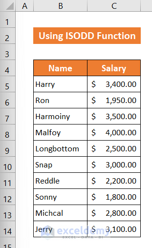
In this similar procedure, we’ll use the ISODD function in place of the ISEVEN function. The ISODD function will highlight the text if the value of the CEILING function is odd.
Steps:
- Select the entire range B4:C14.
- In the Home tab, go to Conditional Formatting > New Rules.

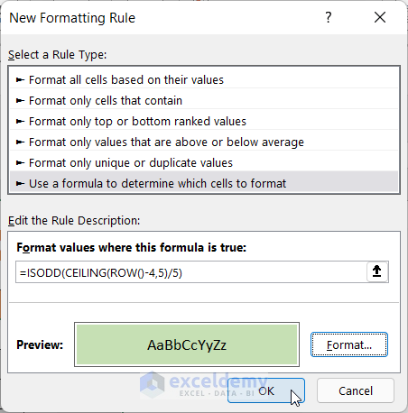
- A new dialog box titled New Formatting Rule will appear.
- Select Use a formula to determine which cells to format.
- Enter the following formula in the empty box beside it:
=ISODD(CEILING(ROW()-4,5)/5)- Click on the Format option.
Another dialog box called Format Cells will appear.
- Go to the Fill tab.
- Change the color, for example to a light green color.
- Click OK to close the Format Cells dialog box.
- Click OK to close the New Formatting Rule box.
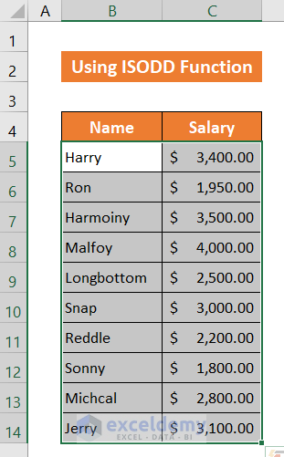
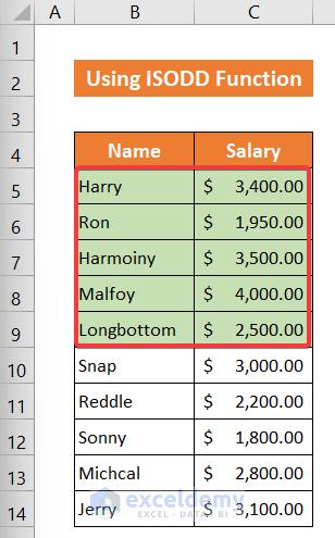
The first 5 rows of the list have our chosen highlight color.
Breakdown of the Formula
For row 5:
ROW(): Returns 5.
CEILING(ROW()-4,5)/5): Returns 1.
ISODD(CEILING(ROW()-4,5)/5): Returns True, meaning the value of the CEILING function is odd, so the ISODD function will highlight the row.
Read More: How to Highlight Row If Cell Is Not Blank
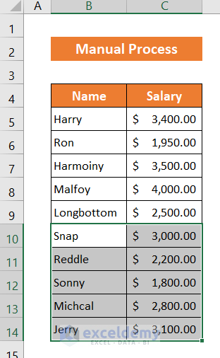
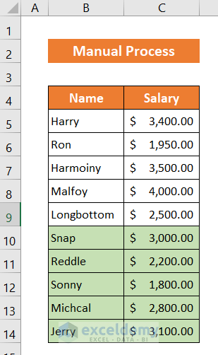
Method 3 – Manually Selecting Every 5 Rows to Highlight
In this method, we will manually select and highlight the last 5 rows of our data list.
Steps:
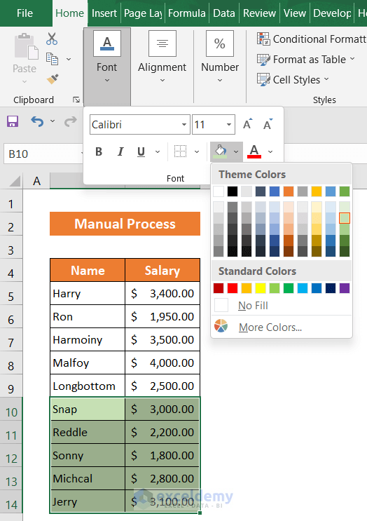
- Select the range B10:C14.
- In the Home ribbon, select the Font > Fill Color icon.
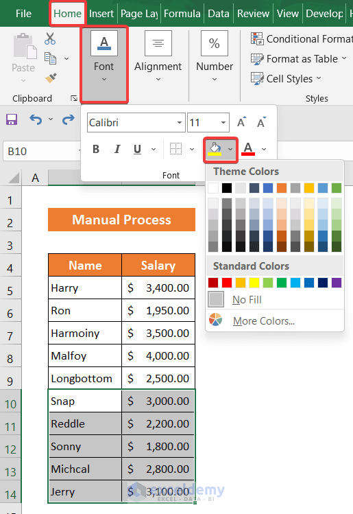
- Choose the Theme Color as, for example, light green.
The last 5 rows are now filled in a light green color.
Read More: How to Highlight Row If Cell Contains Any Text in Excel
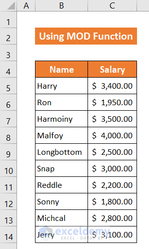
Method 4 – Using the MOD and ROW Functions to Highlight Every 5th Row in Excel
Now we will use the MOD and ROW functions to highlight every 5th row of the dataset.
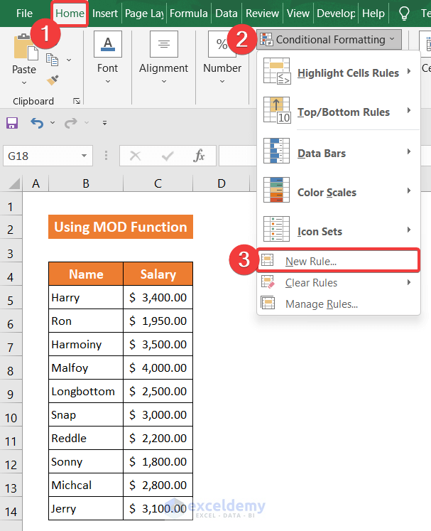
Steps:
- Select the entire range B4:C14.
- In the Home tab, go to Conditional Formatting > New Rules.
A new dialog box titled New Formatting Rule will appear.
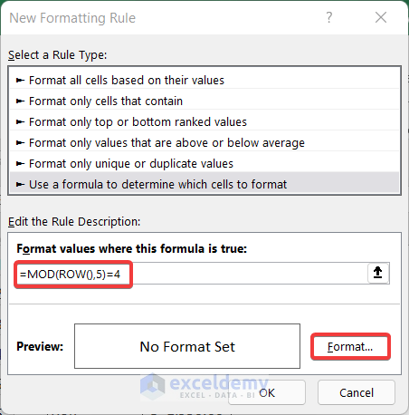
- Select Use a formula to determine which cells to format.
- In the empty box below Format values where this formula is true, enter the following formula:
=MOD(ROW(),5)=4- Click on Format.
- Another dialog box called Format Cells will appear.
- Go to the Fill option.
- Change the white cell color into a light green color.
- Click OK to close the Format Cells dialog box.
- Click OK to close the New Formatting Rule box.

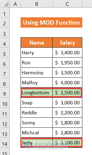
Every 5th row is highlighted with our chosen highlight color.
Breakdown of Our Formula
For row 9:
ROW(): Returns 9.
MOD(ROW(),5)=4: Returns True, which means the remainder value of the ROW function plus 5 is equal to 4, so the function will highlight the row.
Download Practice Workbook
Related Article
<< Go Back to Highlight Row | Highlight in Excel | Learn Excel
Get FREE Advanced Excel Exercises with Solutions!
