How to Highlight Every Other Row in Excel (3 Easy Methods)

In this article, we will see how to highlight every other row in Excel. Some available techniques are applying conditional formatting, using different table styles, and applying Excel VBA code. It’s a good practice to highlight different rows in Excel for better readability. It is quite an easy task to highlight different rows manually in a small table. But when you have to deal with a large table in your worksheet you need to impose a different approach.

Download Practice Workbook

Download this practice workbook to exercise while you are reading this article.

3 Suitable Ways to Highlight Every Other Row in Excel

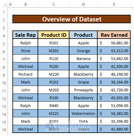
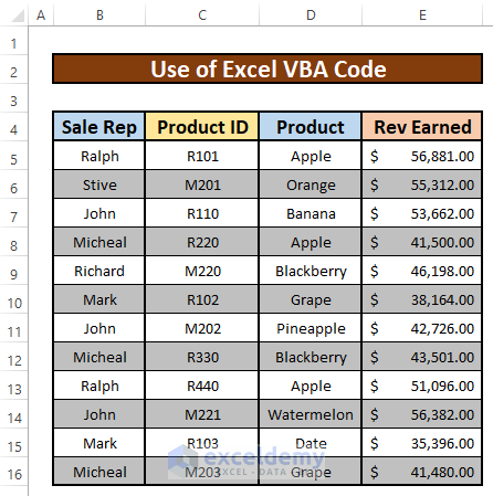
Let’s assume we have an Excel large worksheet that contains the information about several sales representatives of Armani Group. The name of the Products and the Products ID is given in Columns D, and C respectively. We will highlight every other row in Excel using the Conditional Formatting Command, the ISEVEN, ISODD, MOD, ROW functions, and VBA code also. Here’s an overview of the dataset for today’s task.

1. Apply Table Styles to Highlight Every Other Row

To apply different row shading in Excel, you can use different table styles. This is the easiest and fastest approach to highlighting rows. The default automatic filtering and color banding make it easy to highlight different rows in Excel. You need to select the data range and convert it to a table to perform the row highlighting.

There are so many numbers of color stripes available for rows and columns highlighting in the format as a table option. The row shading can be done following the below procedure for different color stripes. Let’s follow the instructions below to learn!

Step 1:

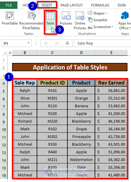
• First of all, select the data range B4 to E16.
• Hence, from the Insert tab, go to,

Insert → Table

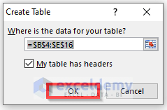
• As a result, a Create Table dialog box will come up. From the Create Table dialog box, press OK.

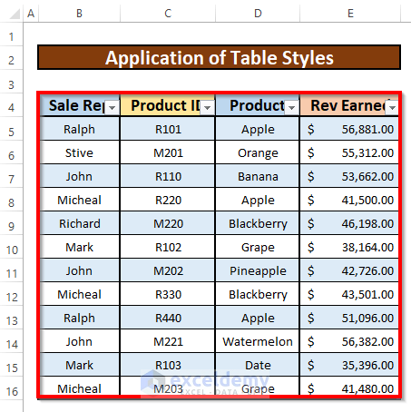
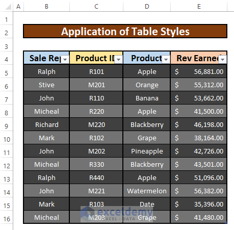
• After that, you will be able to create a table with highlighting default color.

Step 2:

• Excel generates a blue and white pattern table by default. Now if you wish to create your own color patterns for the table you can also do that. For this, you need to format the table. To do that, just click on the Format as Table option from the Styles group under the Home You will find more patterns and colors.

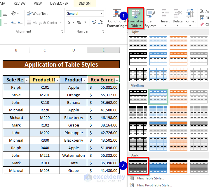
• Hence, you will be able to change the default highlight color of the created table. You can also use the Design option on top of your spreadsheet where you will find the color options with the table style option.

2. Use Conditional Formatting to Highlight Every Other Row

Conditional formatting is a good practice for highlighting or shading a specific row. With the help of conditional formatting, you can highlight different rows according to your choice. Here, we will see the use of two formulas in conditional formatting for highlighting rows.

2.1 Apply ISEVEN Function

Using the ISEVEN function in conditional formatting you can highlight the even rows in a specific range. For example, if you want to highlight the even rows from the range A1: D9, choose the entire range and select the New Rule under Conditional Formatting and use this formula =ISEVEN(ROW()). The procedure is stated below.

Steps:

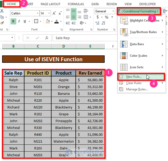
• First, select cells from B5 to B16 to apply the conditional formatting. Then, from your Home tab, go to,

Home → Styles → Conditional Formatting → New Rule

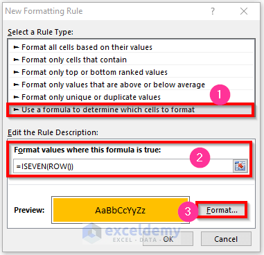
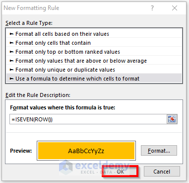
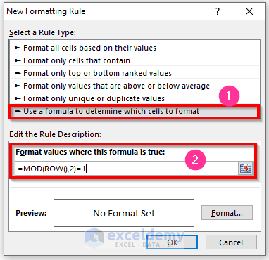
• A dialog box named New Formatting Rule will appear. Follow the steps for the New Formatting Rule dialog box. Firstly, select Use a formula to determine which cells to format from the Select a Rule Type: Secondly, write the below formula in the Format values where this formula is true:. The ISEVEN function is,

• Hence, press the Format option.

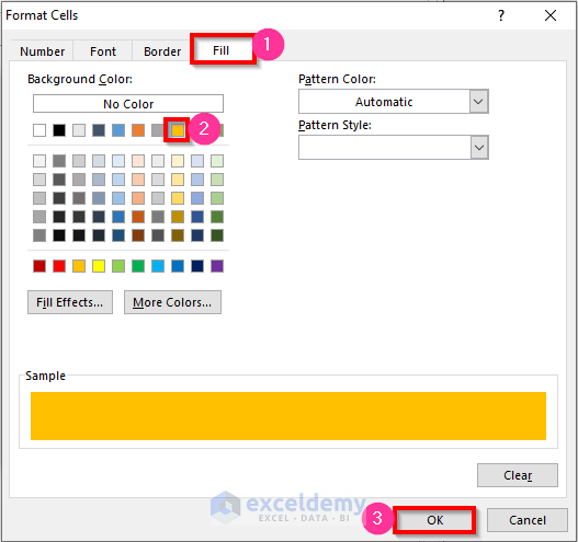
• After clicking on the Format option, a Format Cells dialog box pops up. From that dialog box, firstly, select the Fill Secondly, select any color from the Background Color menu. We have chosen dark yellow. At last, click OK.

• Hence, you will go back to the New Formatting Rule dialog box. Finally, you have to click OK.

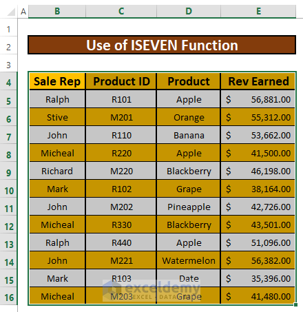
• Finally, you will be able to highlight every other row that has been given in the below screenshot.

2.2 Use ISODD Function to Highlight Every Odd Row

Using the ISODD function in conditional formatting you can highlight the odd rows in a specific range. For example, if you want to highlight the odd rows from the range B5:E16, choose the entire range and select the New Rule under Conditional Formatting and use this formula =ISODD(ROW()). The procedure is stated below.

Steps:

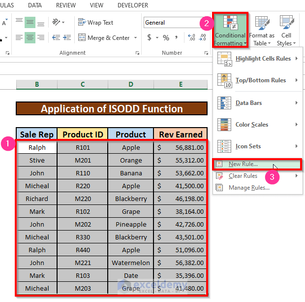
• First, select cells from B5 to B16 to apply the conditional formatting. Then, from your Home tab, go to,

Home → Styles → Conditional Formatting → New Rule

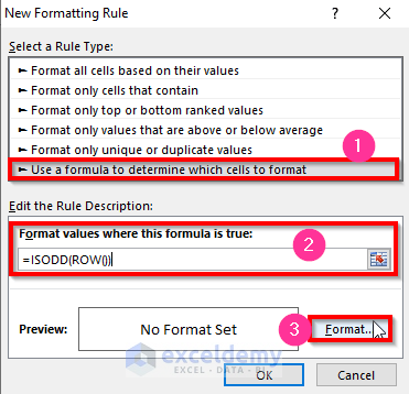
• A dialog box named New Formatting Rule will appear. Follow the steps for the New Formatting Rule dialog box. Firstly, select Use a formula to determine which cells to format from the Select a Rule Type: Secondly, write the below formula in the Format values where this formula is true:. The ISODD function is,

• Hence, press the Format option.

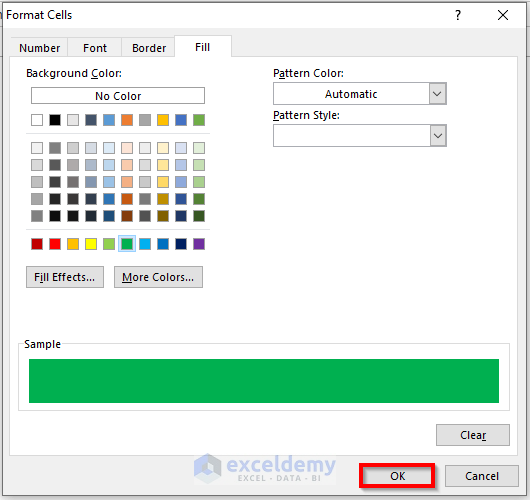
• After clicking on the Format option, a Format Cells dialog box pops up. From that dialog box, firstly, select the Fill Secondly, select any color from the Background Color menu. We have chosen a green color. At last, click OK.

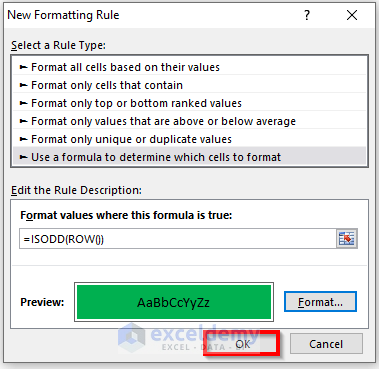
• Hence, you will go back to the New Formatting Rule dialog box. Finally, you have to click OK.

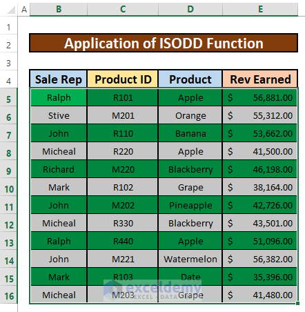
• Finally, you will be able to highlight every odd row that has been given in the below screenshot.

2.3 Formatting in Group Using Multiple Functions in a Single Formula

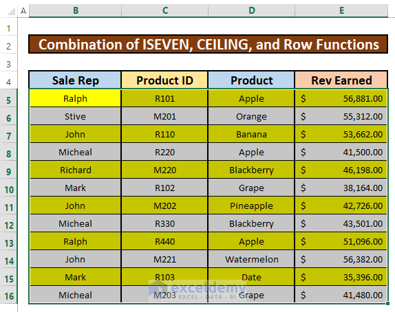
Suppose you need to highlight every other row in a group. You can apply conditional formatting with a formula based on the ISEVEN/ISODD, CEILING, and ROW functions to perform this highlighting. To do that, simply repeat sub-method 1. You can only change the below formula in the New Formatting Rule dialog box to highlight every other row,

• The pictures below show the result that we discussed in this example.

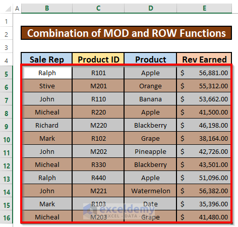
2.4 Combine MOD and ROW Functions to Highlight Rows

Instead of the ISEVEN/ISODD function, we can also use the MOD function to highlight different rows. Like the ISEVEN/ISODD function, this formula also determines whether a row is even or odd-numbered, and then applies the shading accordingly. To highlight every even row, simply repeat sub-method 1. You can only change the below formula in the New Formatting Rule dialog box to highlight every even row,

• The following pictures show the highlighted even rows.

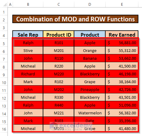
• If you want to highlight the odd rows using the same formula, you can just use a 1 instead of 0 in the above formula. The result and formula stated in the conditional formatting are shown in the below pictures.

• After that, select the Format option to highlight every odd row. We will highlight every odd row with Red color.

3. Run VBA Code to Highlight Every Other Row

For highlighting different rows in excel we can also use the VBA code. Here in this example, we used a VBA code that highlights the even rows. Let’s follow the instructions below to highlight the even rows!

Step 1:

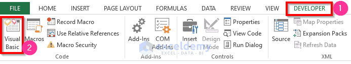
• First of all, open a Module, to do that, firstly, from your Developer tab, go to,

Developer → Visual Basic

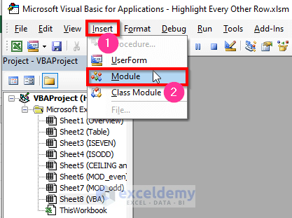
• After clicking on the Visual Basic ribbon, a window named Microsoft Visual Basic for Applications – Highlight Every Other Row.xlsm will instantly appear in front of you. From that window, we will insert a module for applying our VBA code. To do that, go to,

Insert → Module

Step 2:

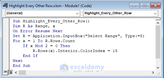
• Hence, the Highlight Every Other Row module pops up. In the Highlight Every Other Row module, write down the below VBA

Sub Highlight_Every_Other_Row()
Dim R As Range, x
On Error Resume Next
Set R = Application.InputBox("Select Range", Type:=8)
For x = 1 To R.Rows.Count
    If x Mod 2 = 0 Then
        R.Rows(x).Interior.ColorIndex = 15
    End If
Next
End Sub

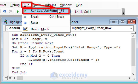
• Hence, run the VBA To do that, go to,

Run → Run Sub/UserForm

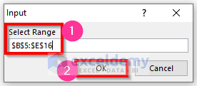
• After running the VBA Code, an Input dialog box pops up. From the Input dialog box, do like the below screenshot.

• Finally, you will be able to highlight every even row which has been given in the below screenshot.

Select Every Other Row in Excel

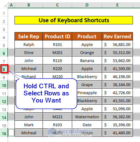
In this section, we will learn how to select every other row in Excel. The easiest and shortest way to select every other row is by using the keyboard and mouse. Let’s follow the instructions below to learn!

Steps:

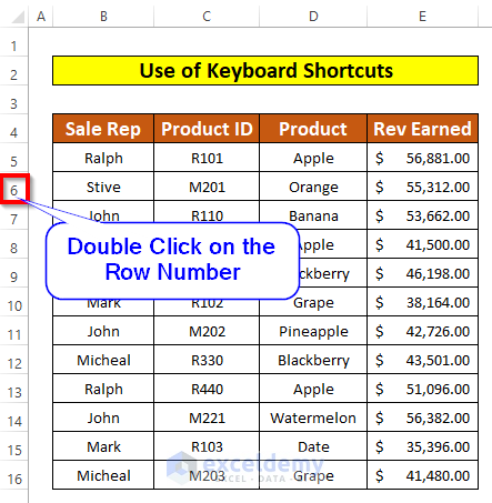
• First, select the row number then double click on the row number by the right side of the mouse.

• Then, it will select the Entire Row.

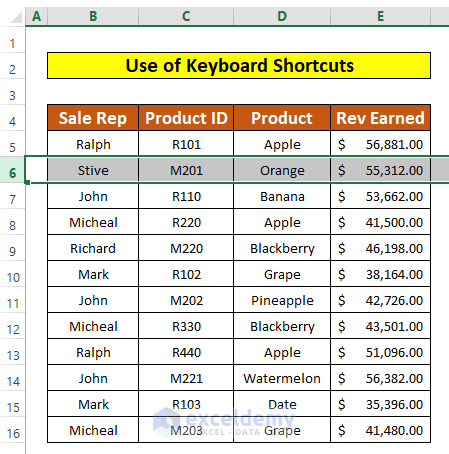
• Now, hold the CTRL key and select the rest of the rows of your choice using the right side of the mouse.

Read More: How To Select All Rows to Below in Excel (3 Easy Methods)

Things to Remember

👉 You can also pop up Microsoft Visual Basic for Applications window by pressing Alt + F11 simultaneously on your keyboard.

👉 If a Developer tab is not visible in your ribbon, you can make it visible. To do that, go to,

File → Option → Customize Ribbon

Conclusion

In this article, we can see different methods to highlight every other row in Excel. Shading/Highlighting different rows in excel improve readability and legibility. While working on a big spreadsheet, it is better to highlight rows.

Hopefully, from now you won`t have any problems while applying color banding in different rows of Excel. This article may help you with the question of how to highlight every other row in excel. If you have applied any other approach to highlight rows, please don’t hesitate to leave a comment.

Related Articles

• Data Clean-up Techniques in Excel: Randomizing the Rows
• How to Delete Blank Rows in Excel (6 Ways)
• Highlight Row If Cell Contains Any Text
• How to Highlight Row If Cell Is Not Blank (4 Methods)