In this article, we will learn how to highlight entire row in Excel with conditional formatting. In Excel, conditional formatting helps users to highlight columns, rows, or cells based on different conditions. Today, we will demonstrate 7 examples. Using these examples, you can easily highlight an entire row with conditional formatting in Excel. So, without further delay, let’s start the discussion.
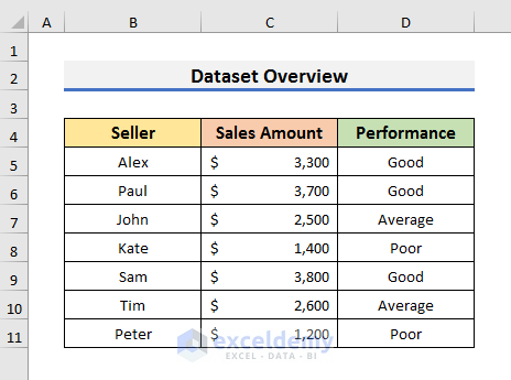
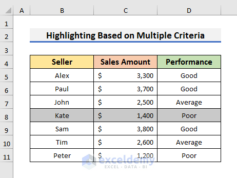
To explain the examples, we will use a dataset that contains information about the Sales Amount, and Performance of some Sellers. We will use conditional formatting based on different criteria and highlight an entire row inside the dataset. You can apply Conditional Formatting based on text, number, multiple criteria, cell value, and many more things. In the following examples, we will show the steps and describe the formula you need to apply conditional formatting correctly.
1. Highlight Entire Row in Excel with Conditional Formatting Based on Text Criteria
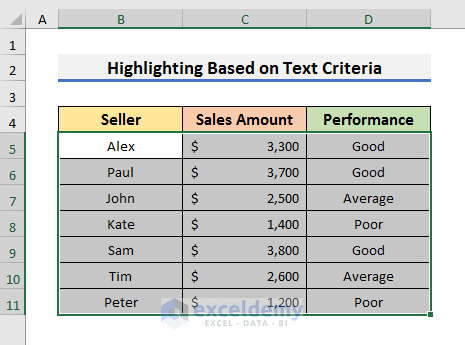
In the first example, we will show how to highlight entire row in Excel with conditional formatting based on text criteria. The steps of this example are simple. Here, we will highlight the entire corresponding row that contains the text Average in Column D. Let’s follow the steps below to learn more about the example.
STEPS:
- In the first place, select the whole dataset without the headers. Here, we have selected the range B5:D11.
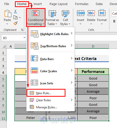
- Secondly, go to the Home tab and select Conditional Formatting. A drop-down menu will appear.
- Select New Rule from there. It will open the New Formatting Rule window.
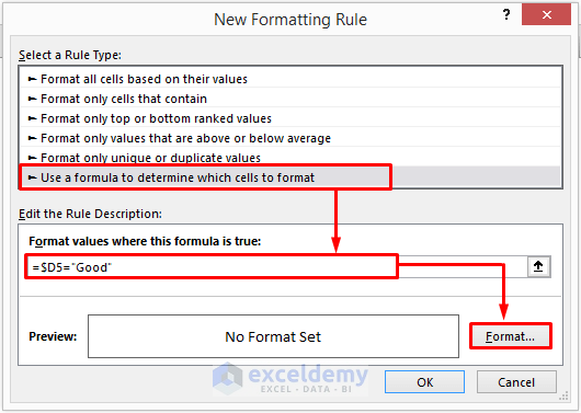
- Thirdly, select ‘Use a formula to determine which cells to format’ from the Select a Rule Type section in the New Formatting Rule box.
- After that, click inside the ‘Format Values where this formula is true’ box and type the formula below:
=$D5="Average"- Now, click on the Format It will open the Format Cells window.

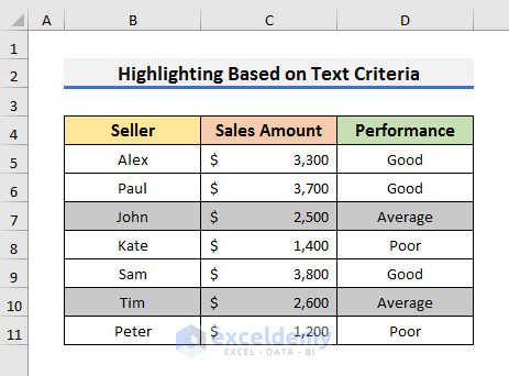
This formula checks each cell in the range B5:D11 if it contains the text Average. We have used a dollar ($) sign to lock column D. But the rows are not locked. That’s why if a cell inside column D contains the word Average, then Excel will highlight the entire corresponding row.
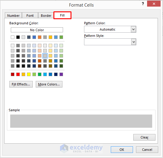
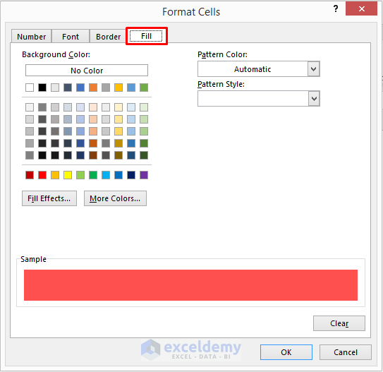
- In the Format Cells window, click on the Fill tab and choose a color from the Background Color section.
- Then, click OK to proceed.

- Finally, you will see Excel has highlighted the rows that contain the word Average in column D.
2. Use Number Criteria in Excel Conditional Formatting to Highlight Entire Row
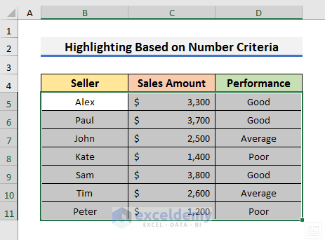
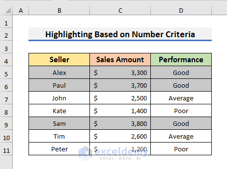
In the second example, we will apply number criteria and see how to highlight entire row in Excel with conditional formatting. Here, we will highlight the corresponding entire row if a cell contains a sales amount greater than $3000. We will use the previous dataset and the same steps as the previous example. Let’s pay attention to the steps below to learn how we can highlight an entire row based on the number criteria.
STEPS:
- Firstly, select the range B5:D11.
- In the second step, select Home >> Conditional Formatting >> New Rule.
- After that, select ‘Use a formula to determine which cells to format’ and type the formula below:
=$C5>=3000- After typing the formula, click on the Format option.

- In the Format Cells window, select a color and click OK to proceed.

- As a result, the rows with a sales amount greater than $3000 are highlighted.
Read More: How to Highlight Every Other Row in Excel
3. Insert Multiple Criteria to Highlight Entire Row in Excel with Conditional Formatting
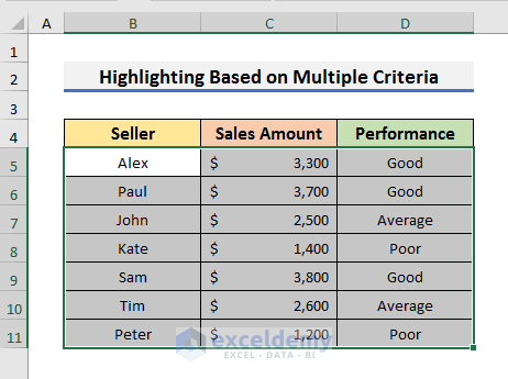
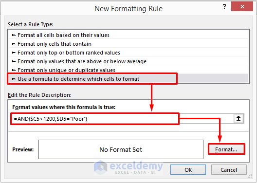
In the previous examples, we used a single criterion in each example. In the 3rd example, I will show you how to highlight entire row in Excel with conditional formatting inserting multiple criteria. For that purpose, we can use AND or OR function. Here, we will highlight an entire row if the sales amount is greater than $1200 and the performance is Poor. To apply Conditional Formatting, both conditions must be satisfied. Let’s follow the steps below to see how we can use multiple conditions.
STEPS:
- In the first place, select the range B5:D11.
- After that, go to the Home tab and select Conditional Formatting >> New Rule.
- The New Formatting Rule window will appear.
- In the New Formatting Rule box, select ‘Use a formula’ option and type the formula below:
=AND($C5>1200,$D5="Poor")- After typing the formula, select Format.
- Now, go to the Fill tab in the Format Cells box and choose a color for highlighting the row.
- Click OK to proceed.
- Finally, you will see results like the picture below.
Read More: How to Highlight Active Row in Excel
4. Apply Conditional Formatting to Highlight Multiple Rows with Different Colors in Excel
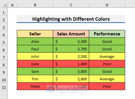
Conditional Formatting has many features and users can perform different operations easily using it. In the previous example, we highlighted the rows with the same color. But in this example, we will use different colors to highlight multiple rows. Again, we will use the same dataset. If the performance of a seller is Good, then the color of the entire row will be green. If the performance is Average, then the entire row color will be yellow. Otherwise, it will be red.
STEPS:
- Firstly, select the range B5:D11.
- Secondly, select Home >> Conditional Formatting >> New Rule.
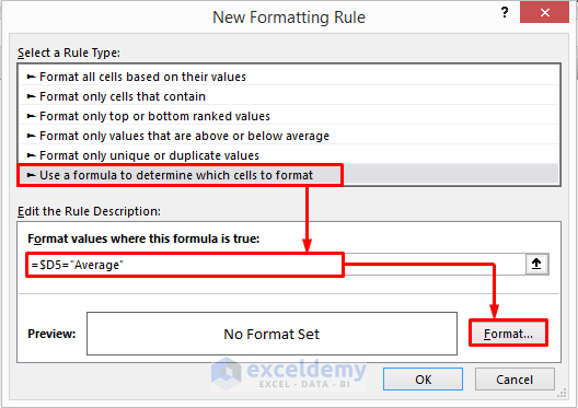
- In the New Formatting Rule box, select ‘Use a formula’ and type the formula below:
=$D5="Good"- Now, click on the Format option.
- After that, go to the Fill tab in the Format Cells box and select the Green color.
- Click OK to move forward.

- Repeat the same steps again and type the formula below in the New Formatting Rule box:
=$D5="Average"- Now, click on the Format option.
- In the Format Cell box, navigate to the Fill tab and select Yellow color this time.
- Click OK to proceed.

- After clicking OK, repeat the steps again.
- In the New Formatting Rule box, type the formula below this time:
=$D5="Poor"- Then, select Format.

- At this moment, select the Fill tab in the Format Cells box and choose Red color.
- Click OK to move forward.
- After completing all the steps successfully, you will see conditional formatting with different colors like the picture below.
Read More: How to Highlight Row If Cell Is Not Blank
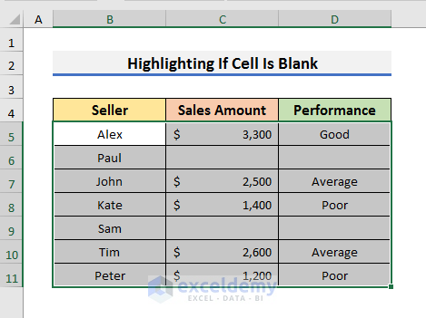
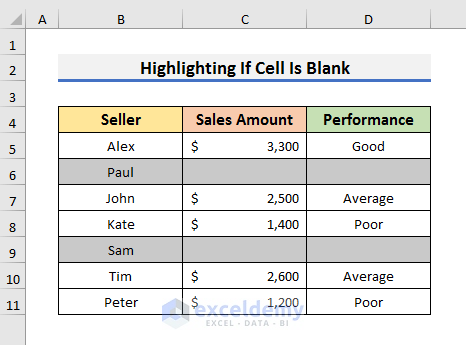
5. Highlight Entire Row If Cell Is Blank with Excel Conditional Formatting
We can also use Conditional Formatting to highlight an entire row in Excel if it contains any blank cells. To do so, we need to use the COUNTIF function in the New Formatting Rule box. Let’s observe the steps below to see how we can implement a formula to highlight an entire row if it stores any blank cells.
STEPS:
- In the beginning, select the range B5:D11.
- Secondly, select Home >> Conditional Formatting >> New Rule.
- In the New Formatting Rule box, click on the ‘Use a formula’ option and type the formula below:
=COUNTIF($B2:$D2)>0- After typing the formula, click on the Format option.
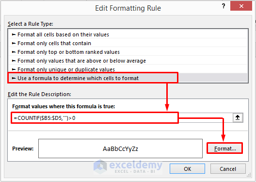
- In the Format Cells window, go to the Fill tab, select a color and then click OK to proceed.

- As a result, you will see Excel has highlighted the corresponding rows with blank cells.
Read More: How to Highlight Every 5 Rows in Excel
6. Use Conditional Formatting to Highlight Entire Row Based on Drop-Down Values
In the 6th example, we will see how to highlight the entire row in Excel with conditional formatting based on the drop-down values. You can see the drop-down list in cell F5 in the dataset below. Here, if we change the value of cell F5 using the drop-down list, then, Excel will dynamically highlight the corresponding row.
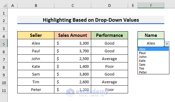
Let’s pay attention to the steps below to see how we can highlight an entire row based on the drop-down values.
STEPS:
- Firstly, select the range B5:D11.
- In the second step, click on the Home tab.
- Then, select Conditional Formatting. A drop-down menu will appear.
- Select New Rule from there. It will open the New Formatting Rule window.
- In the New Formatting Rule box, click on the ‘Use a formula’ option and type the formula below:
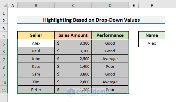
=$B5=$F$5- After typing the formula, click on the Format option.

- At this moment, select the Fill tab in the Format Cells box and choose a color to highlight an entire row.
- Click OK to move forward.

- As a result, you will see Excel has highlighted the corresponding row.

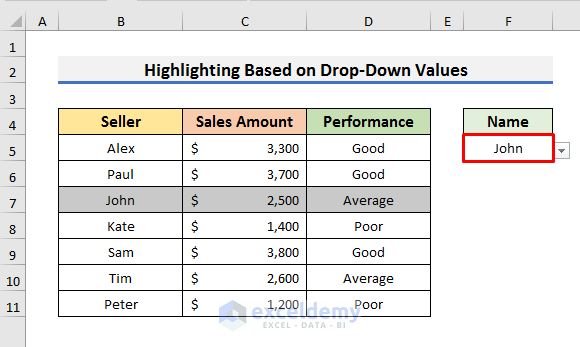
- Now, if you change the value of cell F5 from the drop-down list, the corresponding entire row will be highlighted.
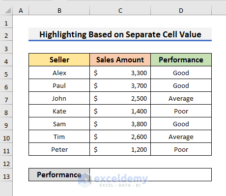
7. Highlight Entire Rows Based on Separate Cell Value
This example is very similar to the previous one. Here, we will show how to highlight the entire row in Excel with conditional formatting based on separate cell values. Suppose, we have a dataset like the picture below. In the dataset, Cell F13 will contain a text or value. Excel will highlight the corresponding row based on that value. In the previous example, we did the same thing from a drop-down list. But, we will change the values manually this time.
Let’s follow the steps below to see how we can implement this example.
STEPS:
- First of all, select the range B5:D11.

- Secondly, select Home >> Conditional Formatting >> New Rule.
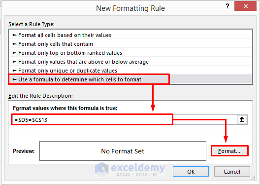
- Thirdly, click on the ‘Use a formula’ option in the New Formatting Rule box and type the formula below:
=$D5=$C$13- After typing the formula, select Format.
- In the Format Cell box, navigate to the Fill tab and select a color from the Background Color section.
- Click OK to proceed.

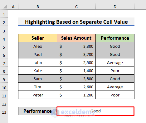
- In the following step, type Good in cell C13 and press Enter.
- Instantly, Excel will highlight the rows with the word “Good”.
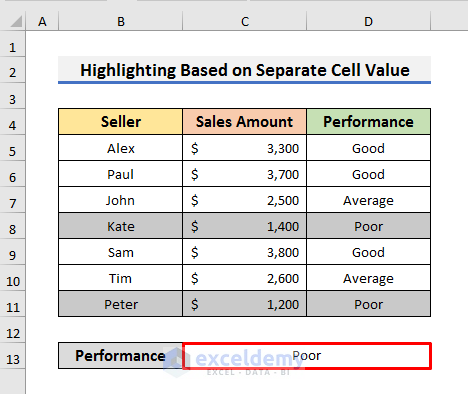
- Finally, if you type another value in cell C13, then the corresponding entire row will be highlighted.
Read More: How to Highlight Row If Cell Contains Any Text in Excel
Download Practice Workbook
You can download the practice book from here.
Conclusion
In this article, we have 7 ideal examples of how to highlight entire row in Excel with Conditional Formatting. I hope this article will help you to perform your tasks efficiently. Furthermore, we have also added the practice book at the beginning of the article. To test your skills, you can download it to exercise.
<< Go Back to Highlight Row | Highlight in Excel | Learn Excel
Get FREE Advanced Excel Exercises with Solutions!
