Here’s a GIF overview of using conditional formatting to highlight rows based on certain values inside them.
How to Highlight Row If the Cell Contains Any Text in Excel
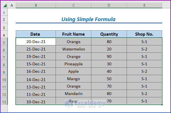
Method 1 – Using a Simple Formula to Highlight a Row If a Cell Contains Any Text
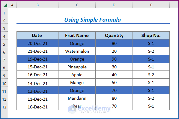
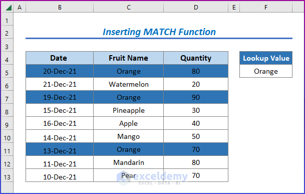
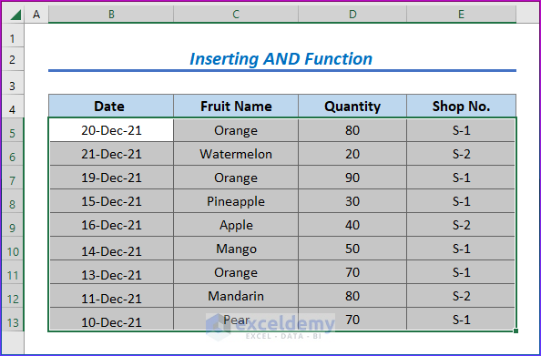
Consider a fruit sales dataset where we want to highlight rows that contain ‘Orange’ as a cell value.
Steps:
- Select the entire dataset (B5:E13).
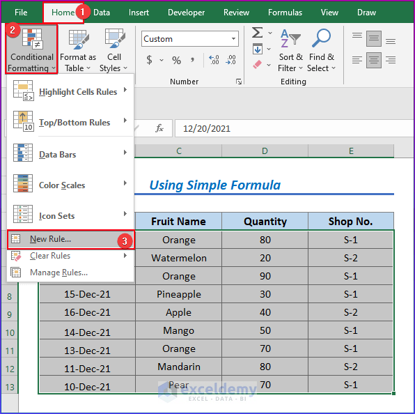
- Go to Home and select Conditional Formatting.
- Choose the New Rule from the Conditional Formatting drop-down.
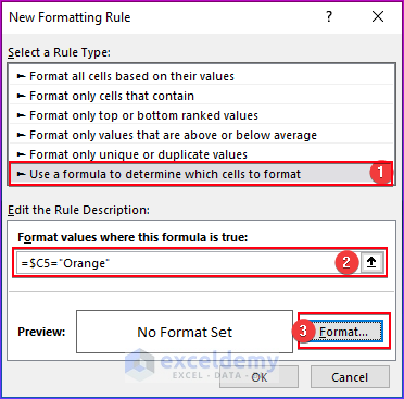
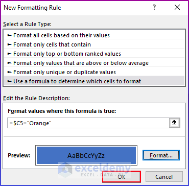
- The New Formatting Rule window will show up. Choose the Use a formula to determine which cells to format option.
- Copy the following formula in the Rule Description box.
=$C5="Orange"
- Click Format.
- Click the Fill tab and choose a fill color.
- Select OK.
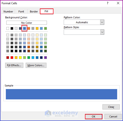
- Click OK again.
- All the rows that contain a cell with value ‘Orange’ will be highlighted.
Read More: How to Highlight Active Row in Excel
Method 2 – Inserting the MATCH Function to Highlight a Row if a Cell Remains any Text
Steps:
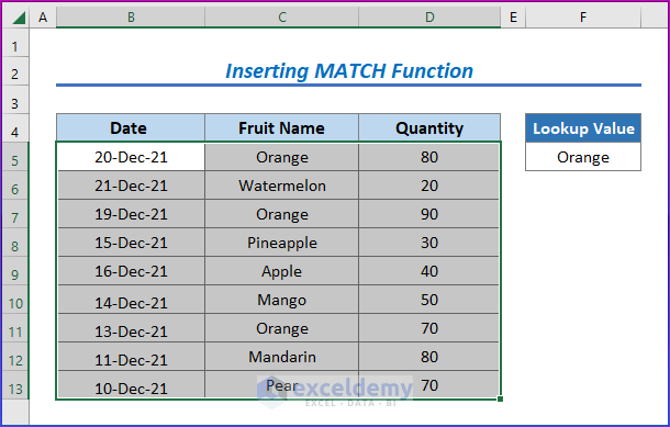
- Select the entire dataset (B5:D13).
- Go to Home and select Conditional Formatting, then choose New Rule.
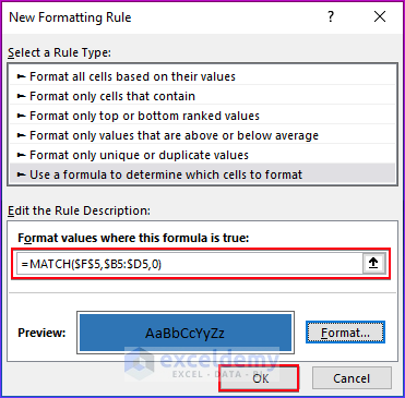
- The New Formatting Rule window will show up. Choose Use a formula to determine which cells to format.
- Copy the following formula in the Rule Description box.
=MATCH($F$5,$B5:$D5,0)
- Click Format, choose the Fill color, and select OK.
- Click OK to close the Formatting rule window.
- All the rows that contain ‘Orange’ in any cell will be highlighted.
How Does the Formula Work?
The MATCH function returns the relative position of an item in an array that matches a specified value in a specified order. The function matches the value of Cell E5 in the range (B5:D5) and thus highlights the corresponding rows containing the text ‘Orange’.
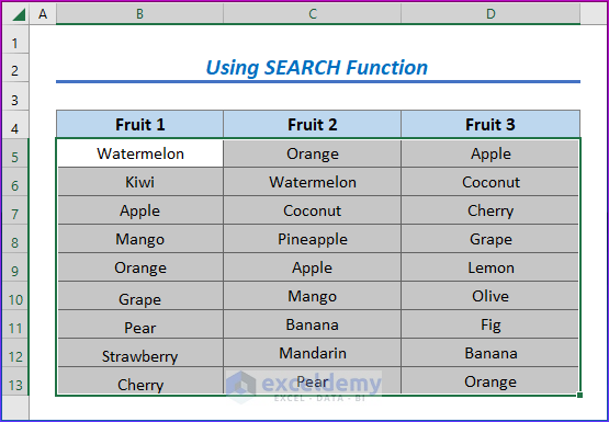
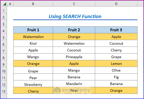
Method 3 – Using the SEARCH Function to Highlight a Row If a Cell Contains Any Text
Here we have a fruit name dataset and will search for a particular fruit to highlight the entire row its in.
Steps:
- Select the entire dataset (B5:D13).
- Go to Home and select Conditional Formatting, then pick New Rule.
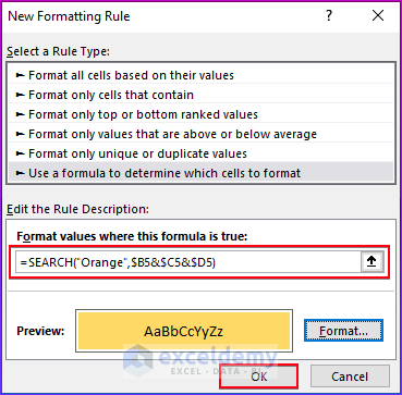
- The New Formatting Rule window will pop up. Select Use a formula to determine which cells to format.
- Copy the following formula in the Rule Description box.
=SEARCH("Orange",$B5&$C5&$D5)
- Click Format, choose the Fill color, and click OK.
- Click OK to apply the formatting rule.
- All the rows that contain ‘Orange’ in any cell will be highlighted.
How Does the Formula Work?
The SEARCH function returns the number of characters at which a specific character or text is first found, reading left to right. The SEARCH function looks for the text ‘Orange’ in Cell B5, C5, and D5. Since a relative reference is used, the function changes for the values in the entire range (B5:D13). Rows containing the text ‘Orange’ are highlighted.
Related Content: How to Highlight Row If Cell Is Not Blank
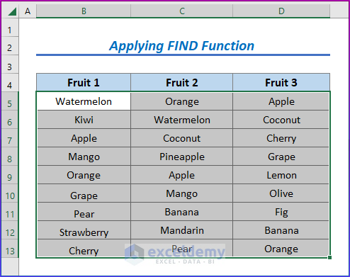
Method 4 – Applying the FIND Function to Highlight a Row for a Case-Sensitive Option
Steps:
- Select the entire dataset (B5:D13).
- Go to Home, select Conditional Formatting, and choose New Rule.
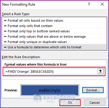
- The New Formatting Rule window will open. Choose Use a formula to determine which cells to format.
- Insert the following formula in the Rule Description box.
=FIND("Orange",$B5&$C5&$D5)
- Click Format, choose a Fill color, and click OK.
- Click OK again.
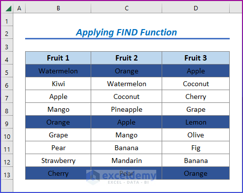
- All the rows that contain ‘Orange’ in any cell will be highlighted. However, rows containing the text ‘orange’ or ‘ORANGE’ are not highlighted as the FIND function is case-sensitive.
Method 5 – Inserting the AND Function to Highlight a Row Based on Two or More Cells
Let’s highlight the sales of Oranges where the Quantity is greater than 70.
Steps:
- Select the entire dataset (B5:E13).
- Go to Home, select Conditional Formatting, and pick New Rule.
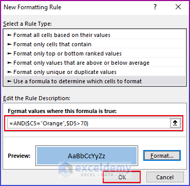
- In the New Formatting Rule window, choose Use a formula to determine which cells to format.
- Enter the following formula in the Rule Description box:
=AND($C5="Orange",$D5>70)
- Click Format, choose a Fill color, and click OK.
- Click OK again.
- All the rows that fulfill Fruit Name: Orange and Quantity: >70 will be highlighted.
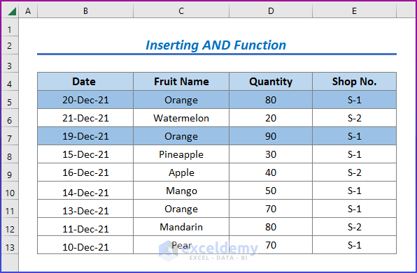
How Does the Formula Work?
The AND function checks whether all arguments are TRUE, and returns TRUE if all arguments are TRUE. Here this function checks both the Fruit Name and Quantity arguments and highlights rows accordingly.
You can use the OR function instead of the AND function if you need only at least one of the requirements to be true.
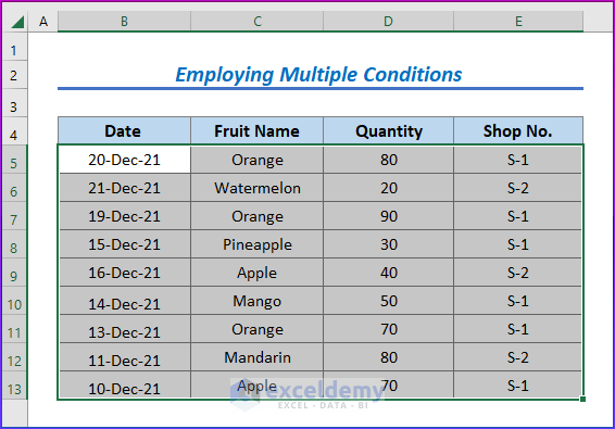
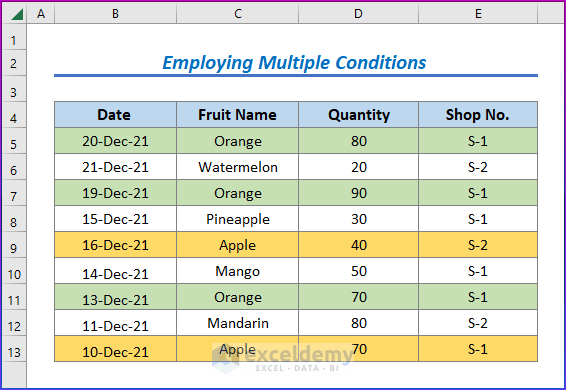
Method 6 – Employing Multiple Conditions to Highlight Rows
Let’s highlight rows that have the text ‘Orange’ or text ‘Apple’.
Steps:
- Select the entire dataset (B5:E13).
- Go to Home, Conditional Formatting, and New Rule.
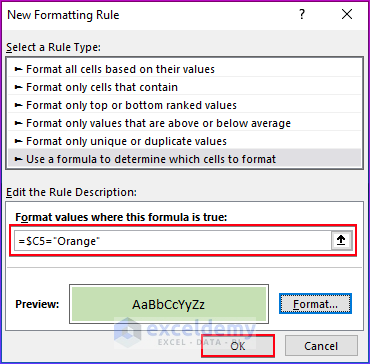
- In the New Formatting Rule window, choose Use a formula to determine which cells to format.
- Copy the following formula in the Rule Description box.
=$C5="Orange"
- Choose Format, choose a Fill color, and click OK.
- Click OK to close the rule window.
- All the rows that contain ‘Orange’ in any cell will be highlighted.
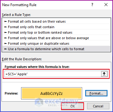
- Repeat the steps to set a new conditions to the existing dataset, using the following formula:
=$C5="Apple"
- Apply a different fill color if you’d like.
- Both conditions will be shown in the dataset.
Read More: How to Highlight Every 5 Rows in Excel
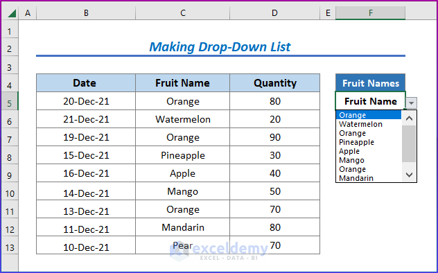
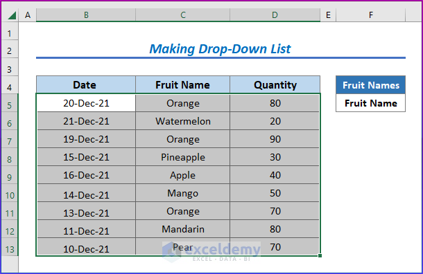
Method 7 – Making a Drop-Down List to Highlight a Row Based on the Selection
Steps:
- Create the drop-down list for the ‘Fruit Name’ column in cell F5.
- Select the entire dataset (B5:D13).
- Choose Conditional Formatting and select New Rule.
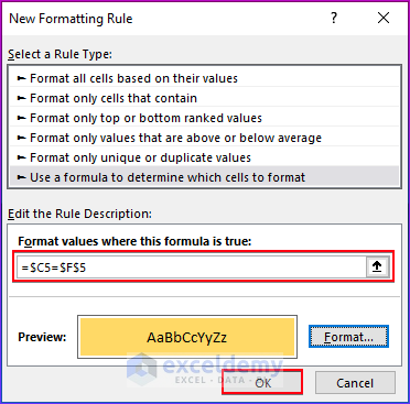
- Select Use a formula to determine which cells to format.
- Use the following formula in the Rule Description box.
=$C5=$F$5
The drop-down value is used as a reference value in the formula.
- Go to Format to choose a Fill color.
- Click OK to close the pop-up windows.
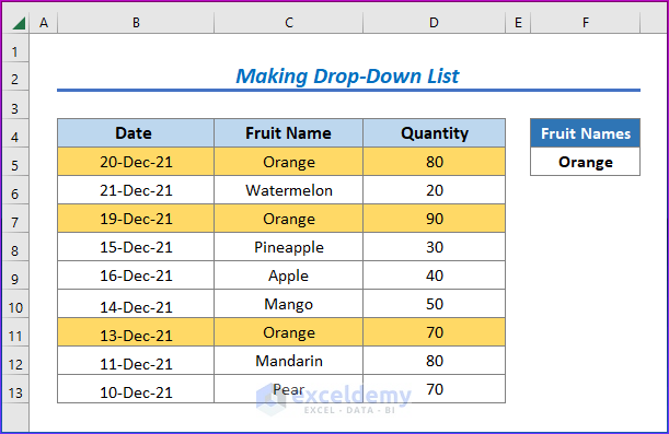
- When we change the fruit name from the drop-down, the highlighting will also change. We have selected ‘Orange’ from the drop-down and all the rows containing ‘Orange’ are highlighted.
Download the Practice Workbook
You can download the practice workbook that we have used to prepare this article.
Related Article
<< Go Back to Highlight Row | Highlight in Excel | Learn Excel
Get FREE Advanced Excel Exercises with Solutions!

Great Job. This article was well written clear, concise, and thorough with different functions and conditions. I was able to find what I needed to do with the explanations in no time.
Thanks for your appreciation @Ed
How to highlight an entire row if a a cell contains any random entry (number/text). Thank you
Hello Euliin,
Thanks for commenting on our website. You can highlight a cell containing any random value with Conditional Formatting. Follow the steps.
Firstly, select the entire row that you want to be highlighted. Then go to the Conditional Formatting and choose New Rule.
Now, New Formatting Rule dialog box appears. Choose Use a formula which cells to format. Write the formula in the box in the Format values where this formula is true.
=OR(ISTEXT(B5),ISNUMBER(B5))And click on Format.
Now, Format Cells appears. Pick a color and hit OK.
Now, again hit OK in the New Formatting Rule box.
Finally, as you see you can highlight the row.