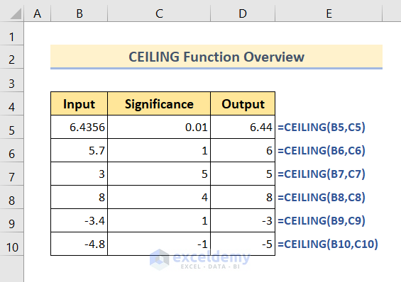
The CEILING function as the name suggests rounds up a number to the nearest top integer or the multiple of the specified significance. If you want to escape from the fraction numbers of your dataset, then the CEILING function is maybe the one, you were actually looking for. To help you in this regard, in this article we will demonstrate the usage of the CEILING function in Excel with 3 suitable examples.
The above screenshot is an overview of the article, representing a few applications of the CEILING function in Excel. You’ll learn more about the methods along with the other functions to use the CEILING function precisely in the following sections of this article.
Download the Practice Workbook
You are recommended to download the Excel file and practice along with it.
Introduction to the CEILING Function
- Function Objective:
The CEILING function is used to round up a number to its nearest upper integer or to the multiple of significance.
- Syntax:
CEILING(number, significance)
- Arguments Explanation:
Argument | Required/Optional | Explanation |
---|---|---|
number | Required | The number that you want to round up. |
significance | Required | This argument instructs you to input either the multiple or the number of digits that you want to show after the point (.). |
- Return Parameter:
Rounded up number according to the significance.
3 Examples to Use the CEILING Function in Excel
We can use the CEILING function to round up different types of numbers such as fraction numbers, negative numbers, and even integer numbers. So without having any further discussion let’s dive straight into the categories.
1. Round up Fraction Numbers Using the CEILING Function
The CEILING function enables us to do a lot, in terms of rounding up the fraction numbers. We can specify the exact number of digits that we want after the point of a fraction number.
As we’ve already known, the CEILING function contains two arguments. The first one is the number that we want to round up and the second one is the specification that tells more details about the rounding up process.
So without having further discussion let’s first have a look, how we can use the CEILING function for the fraction numbers. Later, we will go into further discussion and explanations.
🔗 Steps:
❶ First of all, select cell D5.
❷ After that insert the formula:
=CEILING(B5,C5)
❸ Now press the ENTER button.
❹ Finally drag the Fill Handle icon to the end of the Output column.
After doing all the steps, we will see our fraction numbers have been rounded up to their nearest ceiling values as in the picture below:
The first number is 6.4356 and its corresponding significance is 0.001. As the significance has two digits after the point, the rounded-up numbers will also have two digits after the decimal point. As a result, we can see the output of the ceiling function has become 6.44 which is the immediate round-up value after 6.43.
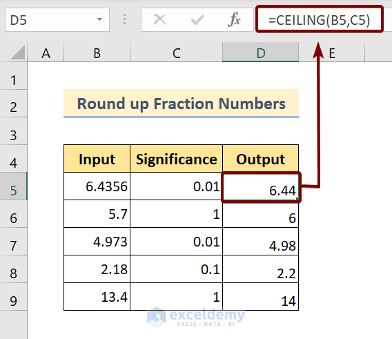
For the second number i.e. 5.7, the significance is 1, which means that there will be no digit after the decimal point. As a result that 5.7 has become 6 after applying the formula.
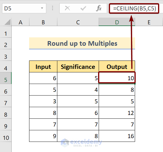
Now you’ve got the main point, right? Then check the rest numbers considering their corresponding significance.
Read More: How to Use ROUNDUP Function in Excel (6 Examples)
2. Round up Numbers to their Multiples Using the CEILING Function
In this section, we will see an amazing feature that the CEILING function provides. We can easily round up numbers to the next multiple of a certain number.
For example, let’s take a number such as 6. Now, let’s our multiple is 5. So the multiples of 5 go like 5,10,15… etc.
As our number here is 6 and the multiples of 5 next to 6 is, so if we use the formula:
=CEILING(B5,C5)
Now follow the steps below to convert a set of numbers to their next multiples according to the specified significance.
❶ Select cell D5.
❷ Insert the formula:
=CEILING(B5,C5)
❸ Press the ENTER button.
❹ Finally, drag the Fill Handle icon to the end of the Output column.
That’s all you need to do. After following each of the above steps, you will see the numbers rounded up as in the image below:
Read More: 44 Mathematical Functions in Excel (Download Free PDF)
Similar Readings
- LARGE function in Excel
- SUMPRODUCT() function in Excel
- How to Use SQRT function in Excel (6 Suitable Examples)
- Use COS Function in Excel (2 Examples)
- How to Use FACT Function in Excel (2 Suitable Examples)
3. Round up Negative Numbers Using the CEILING Function
We can round up negative numbers in one of the two following ways. We can round them up either towards zero or away from zero. If the sign of the significance is positive then they will be rounded up towards zero; otherwise, they will be rounded up away from zero.
🔗 Steps:
❶ Select cell D5.
❷ Insert the formula:
=CEILING(B5,C5)
❸ Press the ENTER button.
❹ Finally, drag the Fill Handle icon to the end of the Output column.
That’s all you need to do. After following each of the above steps, you will see the numbers rounded up as in the image below:
Let’s pick up the second number i.e. -5.7 for illustration. Its significance specified is -1. As the sign of the significance argument is negative, the output will go away from zero. So the output as we can see in the above picture is -6.
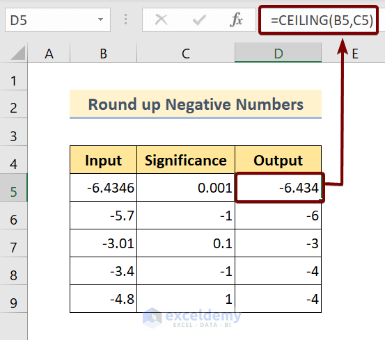
Again for the last number of the list which is -4.8, the specified significance is 1. So the output will proceed towards zero to round up itself using the formula.
As a result, we can see that the output is -4.
Things to Remember
📌 If any of your inserted arguments are nonnumerical, then Excel will return the #VALUE error.
📌 By default, the CEILING function rounds up numbers by adjusting them away from zero (0).
Conclusion
To sum up, we have discussed the usage of the Excel CEILING function with 3 suitable examples. You are recommended to download the practice workbook attached along with this article and practice all the methods with that. And don’t hesitate to ask any questions in the comment section below. We will try to respond to all the relevant queries asap. And please visit our website Exceldemy to explore more.