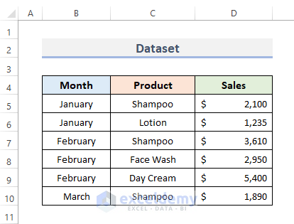
The following dataset contains three months: January, February, and March, and products for three months. Let’s see how to group the dataset by month and summarize the total sales.
Method 1 – Grouping and Summarizing Data with the Subtotal Tool
STEPS:
- The dataset has been sorted by month.
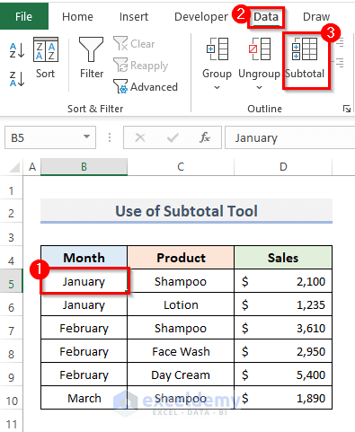
- Select any cell of your dataset. In our case, we selected cell B5.
- Go to the Data tab from the ribbon.
- Click on the Subtotal tool under the Outline category.
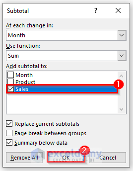
- The Subtotal dialog box will appear.
- Select Month in At each change in: the drop-down section. Select the Sum in Use function: drop-down menu.
- In the Add subtotal to: option, check the Sales box.
- Check the Replace current subtotal and Summary below data box.
- Click OK to complete the procedure.
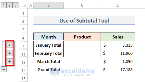
- You will see that the month of January is in a group, and the total sales for January will be calculated below the January group. Similarly, this will group and summarize the February and March months.
- This will also calculate the Grand Total.
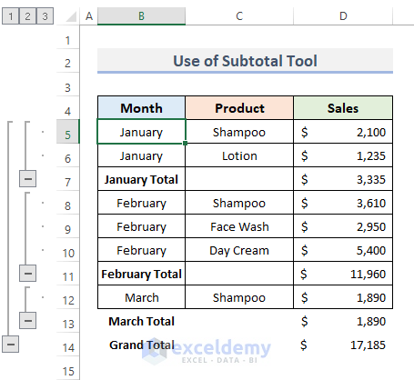
- If you don’t want to display the detailed information, click the minus (–) button. This will hide detailed information about the dataset.
- Undo this by clicking the plus (+) button.
Method 2 – Combine Excel IF and SUMIF Functions to Summarize Data by Group
STEPS:
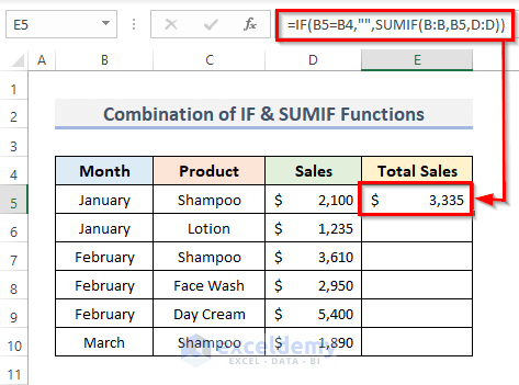
- Select the cell where you want to put the formula.
- Enter the formula into that selected cell.
=IF(B5=B4,"",SUMIF(B:B,B5,D:D))- Press Enter to see the result.
How Does the Formula Work?
- SUMIF(B:B,B5,D:D): B:B is the columns we would like to total depending on, and D:D is the column you would like to total the entries in. Cell B5 is the relative cells we would really like to total depending on. This will calculate the total of the fields.
- IF(B5=B4,””,SUMIF(B:B,B5,D:D)): B4 is the column heading, and cell B5 is the relative cell. If the condition matches, the result will be returned.
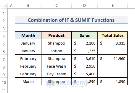
- Drag the Fill Handle down to duplicate the formula over the range. Or, to AutoFill the range, double-click on the plus (+) symbol.
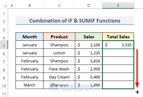
- You can see the sum of data by group.
Method 3 – Categorize and Summarize Data in Excel with a Pivot Table
STEPS:
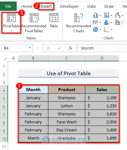
- Select the whole dataset.
- Go to the Insert tab from the ribbon.
- Click on PivotTable.
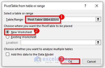
- This will display the PivotTable from table or range dialog box.
- The range will automatically be placed, as we previously selected the data. You can see that selected range in the Table/ Range field under the Select a table or range option.
- In Choose where you want the PivotTable to be placed, select New Worksheet.
- Click the OK button.
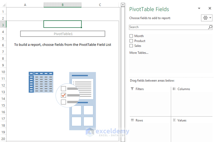
- This will take you to a new sheet where you can organize the pivot table.
- To display the PivotTable Fields, click on any cell in PivotTable1, as shown in the screenshot below.
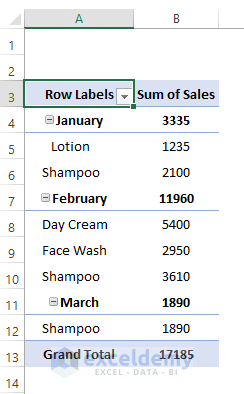
- Place the Month and Product in the Rows field and Sales in the Values field. You can do this by dragging the item.
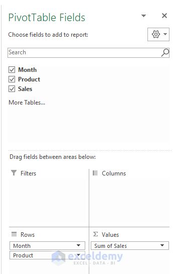
- You can see the table is created in your worksheet. The table is grouped and summarized.
Download the Practice Workbook
Related Articles
- How to Summarize Data by Multiple Columns in Excel
- How to Summarize Data Without Pivot Table in Excel
- How to Create Summary Table in Excel
- How to Create Summary Table from Multiple Worksheets in Excel
- How to Summarize a List of Names in Excel
- How to Make Summary in Excel From Different Sheets
<< Go Back to Summarize Data In Excel | Data Analysis with Excel | Learn Excel
Get FREE Advanced Excel Exercises with Solutions!


its very detailed, informative and helpful.
Hello Calvet,
You are most welcome. Thanks for your appreciation. We are glad to her that you found our article helpful and informative. Keep learning Excel with ExcelDemy!
Regards
ExcelDemy