How to Summarize a List of Names in Excel (5 Ways)

Method 1 – Using the ‘Remove Duplicates’ Command

Steps:

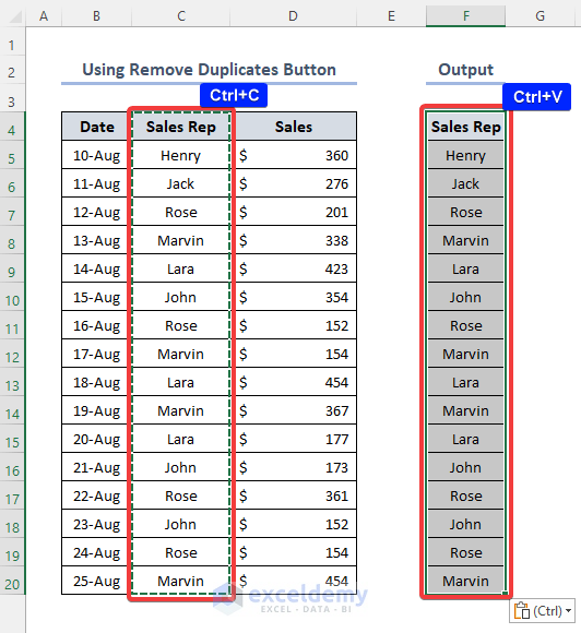
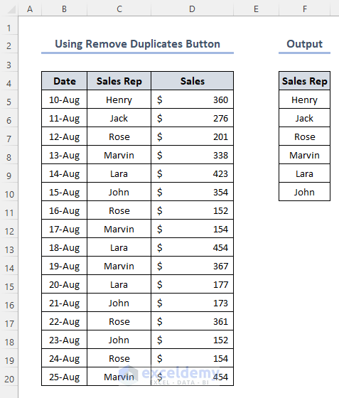
• Copy the ‘Sales Rep’ column and paste it below ‘Output’.

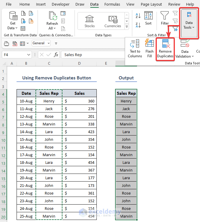
• To remove repeated names from the column, go to Remove Duplicates, found in Data Tools under the Data tab.

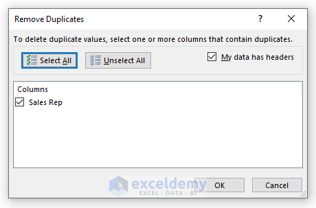
• Remove Duplicate dialog box will pop up.
• Click OK.

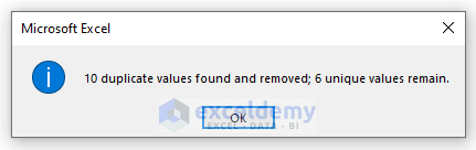
• The number of duplicated values found and removed will be shown in a pop-up box, and the remaining unique values will be shown.

• The unique employees are below the Output column.

Read More: How to Summarize Text Data in Excel

Method 2 – Summarizing a List of Names with Number of Occurrences

Steps: 

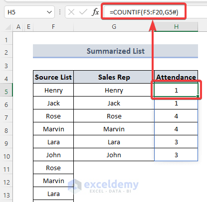
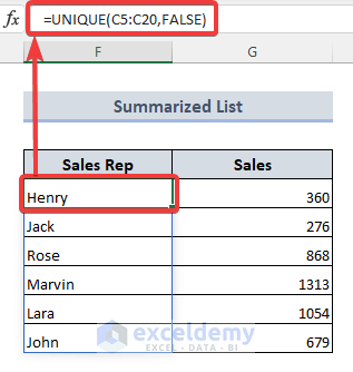
• Find unique employees through the UNIQUE function in Excel that is available in Microsoft 365.

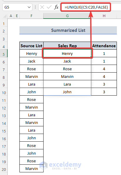
• Use the the COUNTIF function to find their repeated presence in the Sales Rep column like in the image below.

Read More: How to Summarize Data by Multiple Columns in Excel

Method 3 – Summarizing a Name List with the Consolidation Tool

Steps:

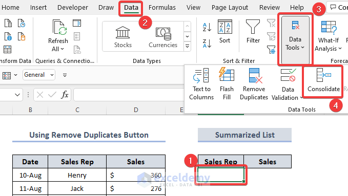
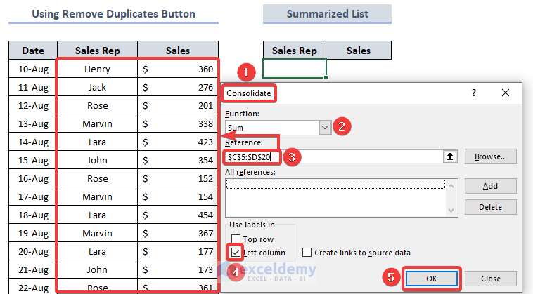
• Select Consolidate in Data Tools under the Data tab to summarize a list of names and their corresponding sales volume.

• A consolidated pop-up will appear.
• In this box, select both columns that we want to summarize.
• Mark the Left Column under Use Labels in.
• Click OK.

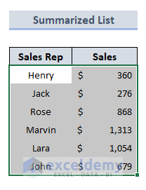
• The final summarized list is shown in the picture below.

Read More: How to Make Summary in Excel From Different Sheets

Method 4 – Applying UNIQUE and SUMIFS Functions

Steps:

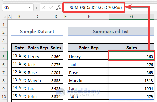
• Use the UNIQUE function. This function will remove any repeated names from the Sales Rep column.

• SUMIFS will sum up all values against repeated names and show them with their unique names.

Read More: How to Create Summary Table in Excel

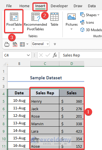
Method 5 – Utilizing the Excel Pivot Table

Steps:

• To pivot any dataset, click the Insert tab
• Click Pivot Table.  

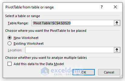
• In the ‘Pivot Table from table or range’ pop-up, click OK to open up a new worksheet for the pivot table.

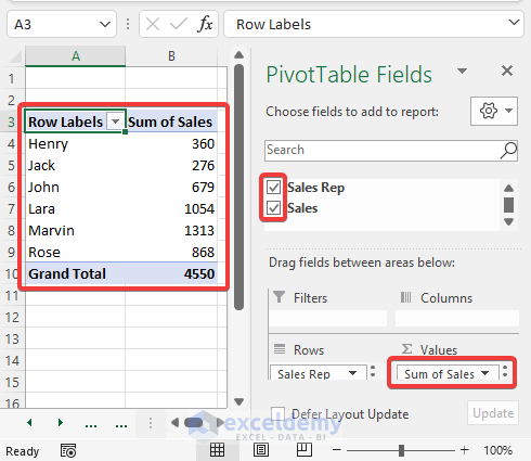
• If we markup both the Sales Rep and Sales columns and values as a sum-up form. The pivot table below will appear. It is good to go for analyzing data for a list of names in Excel.

Read More: How to Summarize Data Without Pivot Table in Excel

Download the Practice Workbook

You can download the practice workbook from the following link.

Related Articles

• How to Summarize Subtotals in Excel
• How to Create Summary Table from Multiple Worksheets in Excel
• How to Group and Summarize Data in Excel
• How to Create a Summary Sheet in Excel

<< Go Back to Summarize Data In Excel | Data Analysis with Excel | Learn Excel