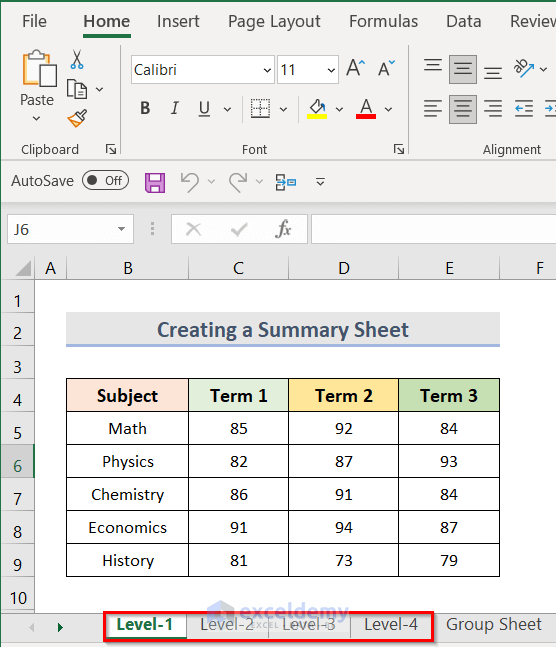
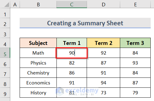
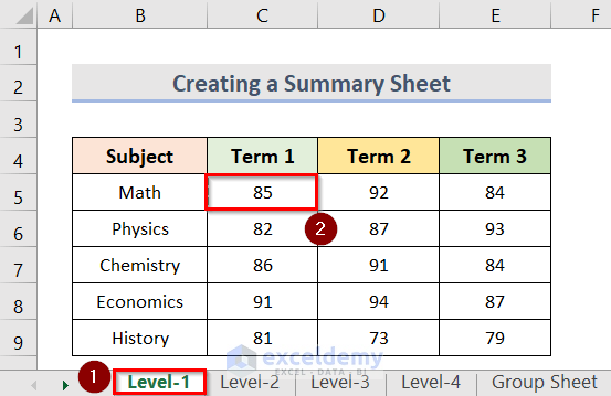
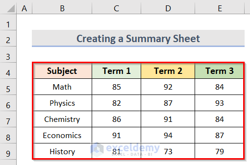
Consider an Excel workbook that contains 4 worksheets named Level-1, Level-2, Level-3 and Level-4, respectively. Each worksheet contains a dataset (B4:E9) that has the Marks of a student in different Subjects for 3 Terms. We will show 4 quick methods to create a summary sheet of these worksheets.
Method 1 – Create a Summary Sheet Using Automatic Update from the Group Sheet Feature
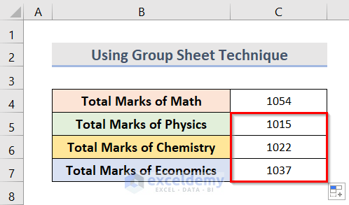
Let’s calculate the total marks of Math, Physics, Chemistry, and Economics at all 4 levels.
Steps:
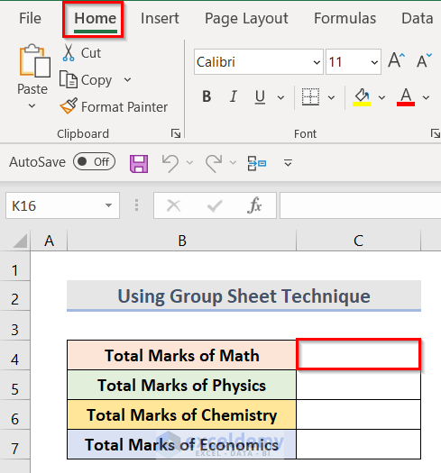
- Open a new worksheet and create a dataset (B4:C7) like the screenshot below.
- Select the cell next to the cell of Total Marks for Math.
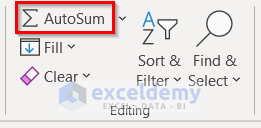
- Go to the Home tab.
- Go to the Editing group and click on the AutoSum option.
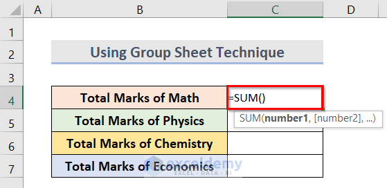
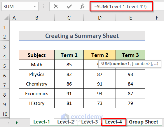
- The SUM function will automatically appear in the cell just like the screenshot below.
- Go to the Level-1 sheet tab, hold the Shift key, and click on the Level-4 sheet tab.
![]()
- Consequently, all the worksheets from Level-1 to Level-4 will be selected. We can also see the selection in the Formula Bar of the screenshot below.
- Select the cell range C5:E5. See the Formula Bar of the screenshot below.
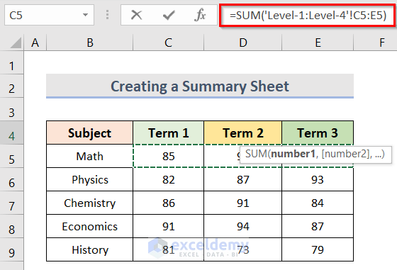
- Hit Enter to get the result.
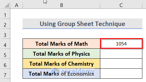
- Drag the fill handle to find the summation of the rest of the Subjects.
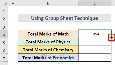
- We can see all the summations in the screenshot below.
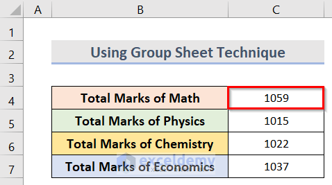
- Change the Marks of Math of Term 1 to 90 to see if it automatically updates the summation.
- We can see that the summation is also updated to 1,059.
Read More: How to Group and Summarize Data in Excel
Method 2 – Insert Excel VBA to Form a Summary Sheet with Hyperlinks
Steps:
- Create a new worksheet and select a blank cell (B4) in it.

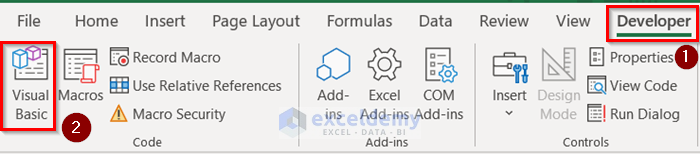
- Go to the Developer tab.
- Go to the Code group and click on Visual Basic.
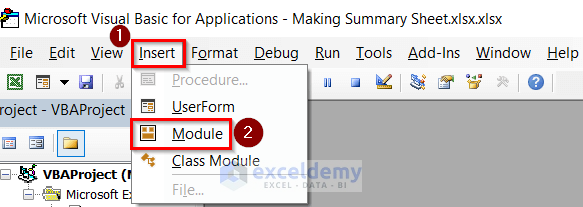
- When the Microsoft Visual Basic for Applications window appears, go to Insert and select Module.
- Insert the following code in the code window:
Sub SummarySheet()
Dim s As Worksheet
Dim c As Range
For Each s In ActiveWorkbook.Worksheets
If ActiveSheet.Name <> s.Name Then
ActiveCell.Hyperlinks.Add Anchor:=Selection, Address:="", SubAddress:= _
"'" & s.Name & "'" & "!A1", TextToDisplay:=s.Name
ActiveCell.Offset(1, 0).Select
End If
Next s
End Sub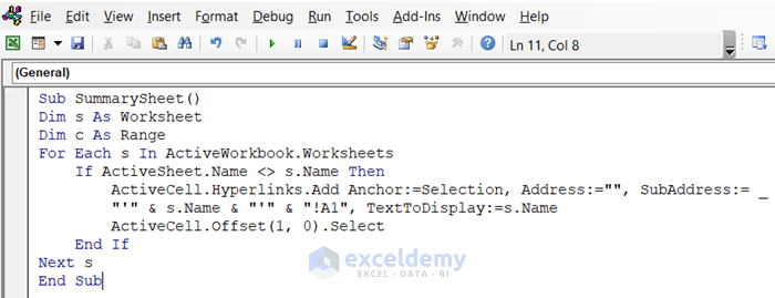
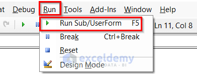
- Go to Run and select Run Sub/UserForm.
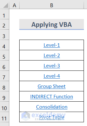
- The hyperlinks of all the worksheets of the Excel workbook will be added to the desired worksheet. By clicking on any hyperlink, Excel will jump to that sheet.
Method 3 – Prepare a Summary Sheet Using the Consolidation Tool
Steps:
- Select a blank cell (C4) in a new worksheet.
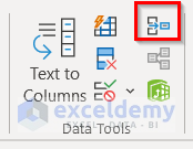
- Go to the Data tab.
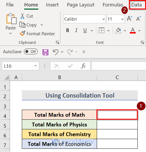
- Go to the Data Tools group and select the Consolidate option.
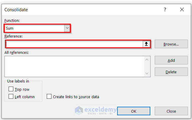
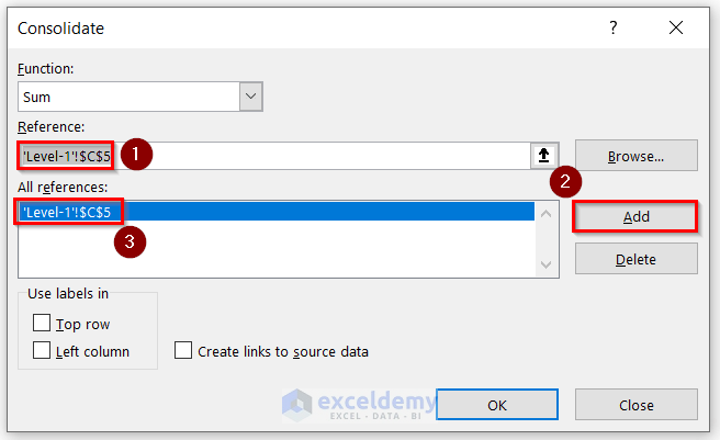
- A Consolidate window will pop up. If you want the sum of the values of the worksheets, select Sum from the Function dropdown. Use other functions as necessary.
- Select the Reference box.
- Click on the Level-1 sheet tab and select cell C5.
- The reference of the cell will be added to the Reference box.
- Click on Add, and the reference will be inserted in the All references box.
- Click on the Level-2 sheet tab and we will see that the cell (C5) that we previously added is already selected.
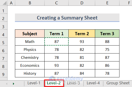
- Go to the Consolidate window again and add this cell reference as well.
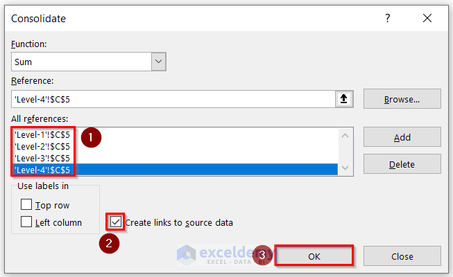
- Repeat for all other references you need.
- Check Create links to source data to automatically update any change of the source data.
- Click on OK.
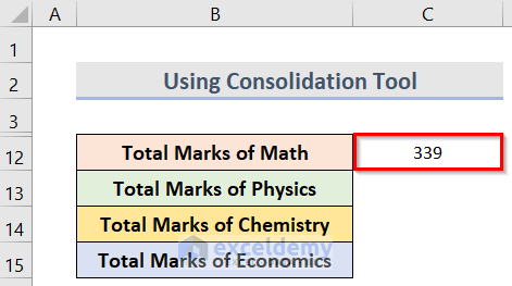
- This sums up values from multiple worksheets.
Read More: How to Make Summary in Excel From Different Sheets
Method 4 – Use an Excel Pivot Table to Summarize Multiple Worksheets
Steps:
- Select a blank cell (B4) in a new worksheet.
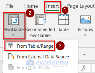
- Go to the Insert tab and click on PivotTable.
- Select From Table/Range from the dropdown.
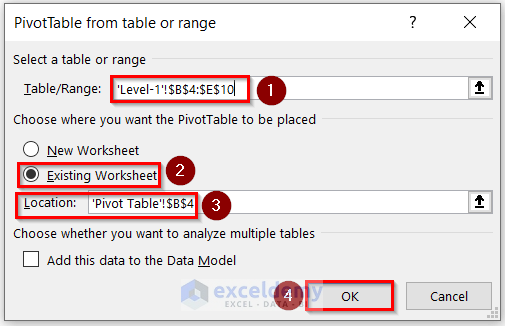
- A window named PivotTable from table or range will open. Go to the Table/Range box.
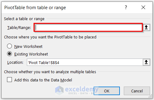
- Select the desired table.
- The reference of the table will be added to the Table/Range box.
- Choose the Existing Worksheet and check the Location of the table in the worksheet.
- Click on the OK button.
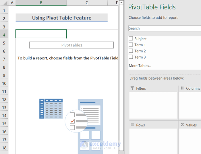
- We will see a Pivot Table area and a section named PivotTable Fields in the worksheet.
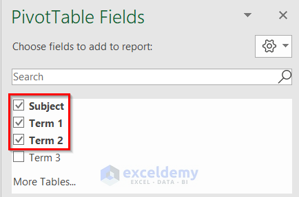
- Select the column headings of the table that you want to insert here. For example, we selected Subject, Term 1, and Term 2.
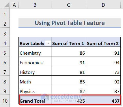
- We will see the contents of the column headings and also the summation of the values in each column. The Pivot Table feature has automatically calculated the summation.
- If you want the average of the column values, select the cell (C10).
- Go to the PivotTable Fields section on the right side of the sheet.
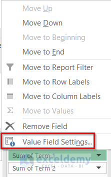
- Go to Values and click on the dropdown arrow of the heading.
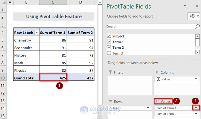
- Click on Value Field Settings.
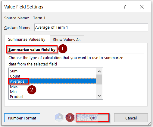
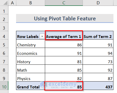
- The Value Field Settings window will open up. Go to Summarize value field by and select Average.
- Click OK.
- This finds the Average of the column.
Read More: How to Summarize Data Without Pivot Table in Excel
Download the Practice Workbook
Download the practice workbook from here.
Related Articles
- How to Summarize Subtotals in Excel
- How to Create Summary Table in Excel
- How to Summarize a List of Names in Excel
- How to Summarize Text Data in Excel
- How to Summarize Data by Multiple Columns in Excel
- How to Create Summary Table from Multiple Worksheets in Excel
<< Go Back to Summarize Data In Excel | Data Analysis with Excel | Learn Excel
Get FREE Advanced Excel Exercises with Solutions!
