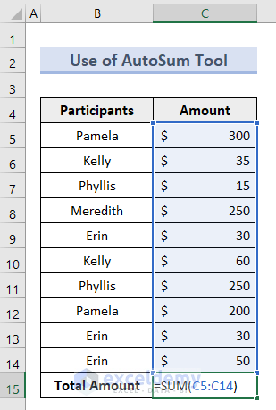
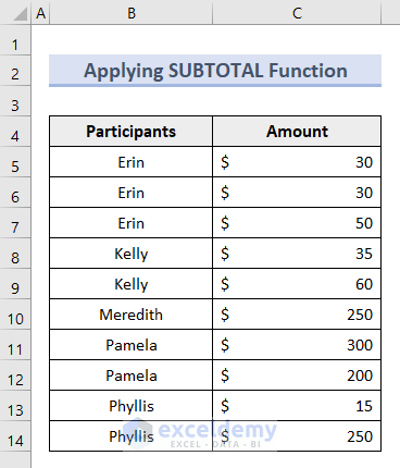
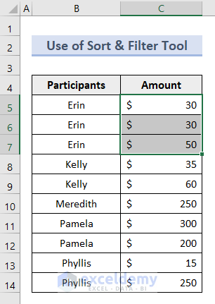
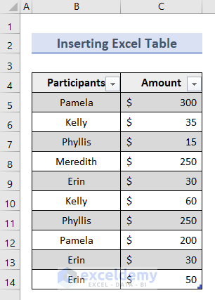
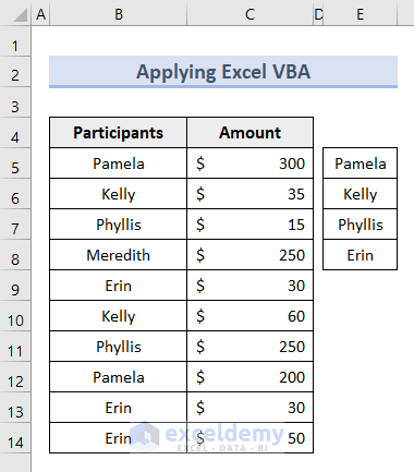
The sample dataset shows trip spending for five people, with repeated entries in the Participants column indicating they had multiple transactions. We will sum up the spending.

Method 1 – Use the AutoSum Tool to Summarize Data in Excel
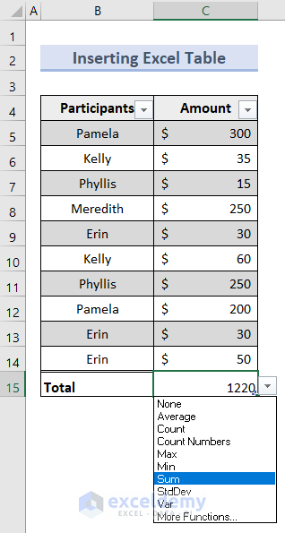
- Select cell C15 because we want the output in this cell.
- Go to the Home tab and select AutoSum under the Editing group.

- You will see that cell C15 is already showing the SUM formula with the reference cell.
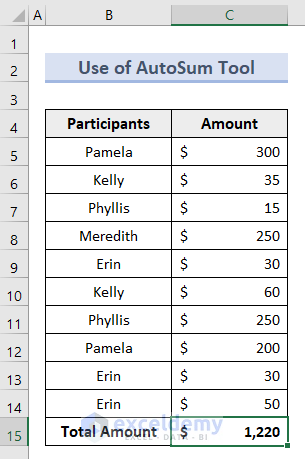
- Press Enter.
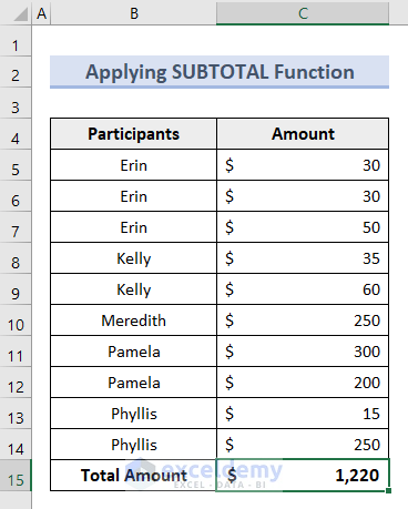
- You will get the total of the spent amounts.
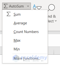
- You can also get the information on average, minimum, or maximum amounts from the dataset by clicking on the options from the drop-down below:
Read More: How to Create a Summary Sheet in Excel
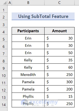
Method 2 – Summarize Data Without a Pivot Table Using Subtotal Feature
- Organize the dataset according to the names. You can use the Sort option for that.
- Select the cell range B4:C14.
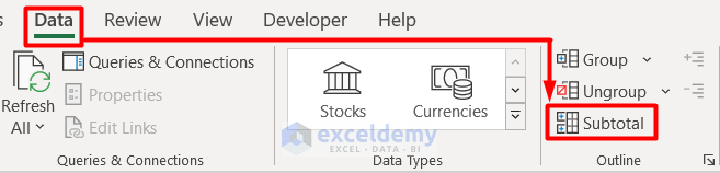
- Go to the Data tab and select Subtotal under the Outline group.
- You will see the Subtotal window pop up.
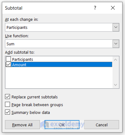
- Put Participants in the At each change in box.
- Insert Sum in the Use function section.
- Check the Amount box.
- Press OK.
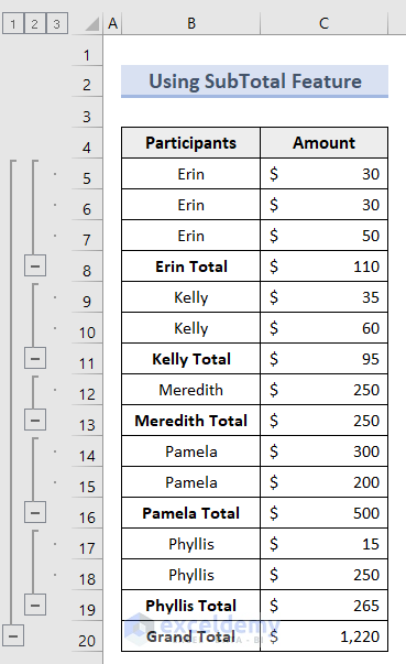
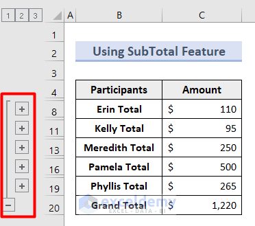
- You can use the Plus (+) and Minus (–) icons to toggle the original cells:
Read More: How to Summarize Text Data in Excel
Method 3 – Apply the SUBTOTAL Function to Add Data in Excel
- Sort the dataset by the name in the first column.
- Insert this formula in cell C15.
=SUBTOTAL(9,C5:C14)The first argument, 9, applies the SUM function while including hidden rows within the range.
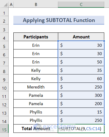
- Press Enter.
Read More: How to Summarize Subtotals in Excel
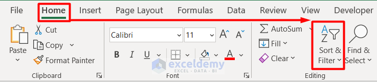
Method 4 – Data Summarizing with the Sort & Filter Tool
- Select cell range B4:C14.
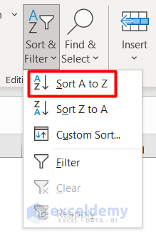
- Go to the Home tab and click on Sort & Filter.
- Select Sort A to Z from the drop-down section.
- The names are sorted in alphabetical order.

- Select consecutive cells that share a name value. We selected the cell range C5:C7.

- Select the Filter option under the Sort & Filter section.
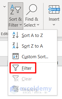
- You will see arrows on the dataset titles.
- Click on the arrow for Participant.
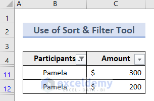
- Select any name to filter. We selected Pamela.

- Press OK.
- You can see only the selected names and their relevant values.
Read More: How to Summarize a List of Names in Excel
Method 5 – Summarize Data with an Excel Table
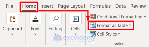
- Go to the Home tab and select Format as Table under the Styles section.
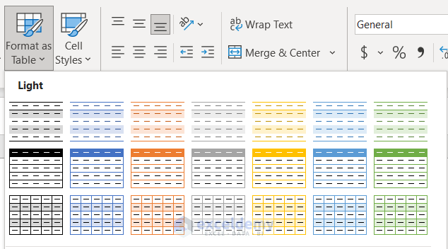
- You will see numerous types of tables to choose from. Choose one.
- You will be directed to the Create Table window.
- Insert the cell range B4:C14 and hit OK.

- Here’s a sample table.
- Select any cell inside it to enable the Table Design tab on the ribbon.
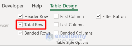
- Go to the Table Design tab and check the Total Row box.
- You will get a new row for the total value with a filter icon beside it.
- Select any option from the drop-down to get a subtotal for that person.
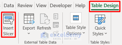
Method 6 – Use a Slicer to Get the Subtotal in the Worksheet
- Create a table following Method 5.
- Go to the Table Design tab and select Insert Slicer.
- You will see the Insert Slicers window asking for the option for creating a slicer.
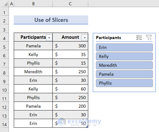
- Select the option Participant and press OK.

- You will get the participant list in a series of buttons.
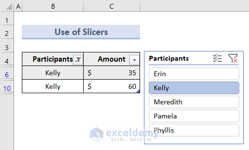
- Select any one of them and you will get the summarized output:
Method 7 – Insert the SUMIF Function to Sum Data Without a Pivot Table
- Create a new table with the same titles on the right.
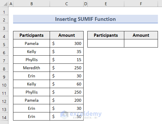
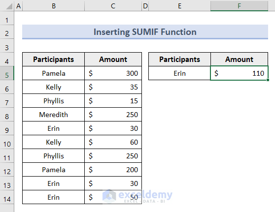
- We want to know the amount spent by Erin. We inserted that name in cell E5.
- Insert this formula in cell F5.
=SUMIF(B5:B14,E5,C5:C14)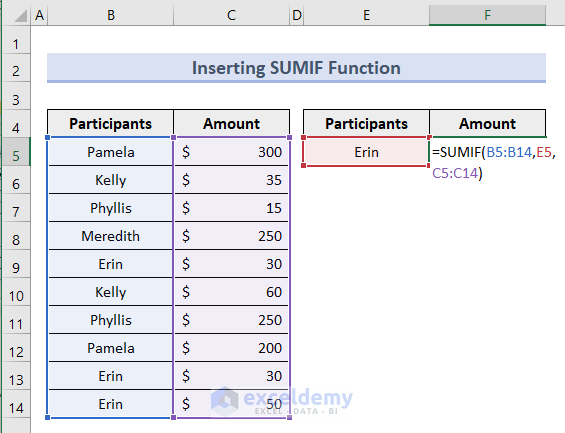
- Press Enter.
Note: You can also apply the IF function with the combination of the SUMIF function to get the same value. The formula will be:
=IF(B9=B4,””,SUMIF(B:B,B9,C:C))
Read More: How to Group and Summarize Data in Excel
Method 8 – Apply Descriptive Statistics to Summarize Data in Excel
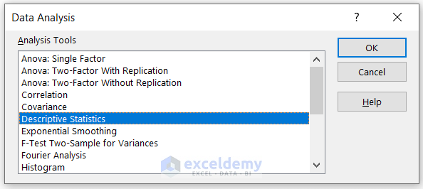
- Go to the Data tab and click on Data Analysis.
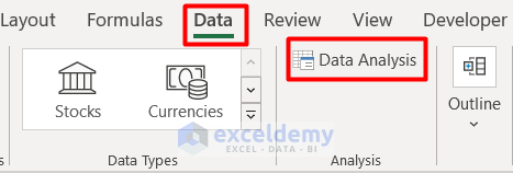
- Select Descriptive Statistics among the Analysis Tools and hit OK.
- Insert the Input and Output Range.
- Check the Summary Statistics box.
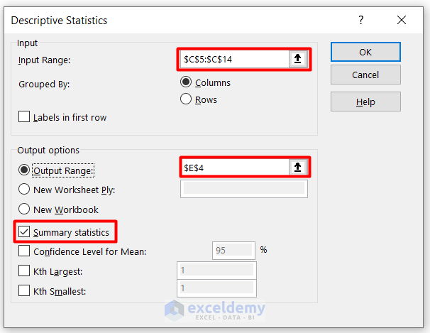
- Press OK.
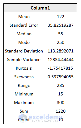
- You will see the detailed statistics of the numeric values.
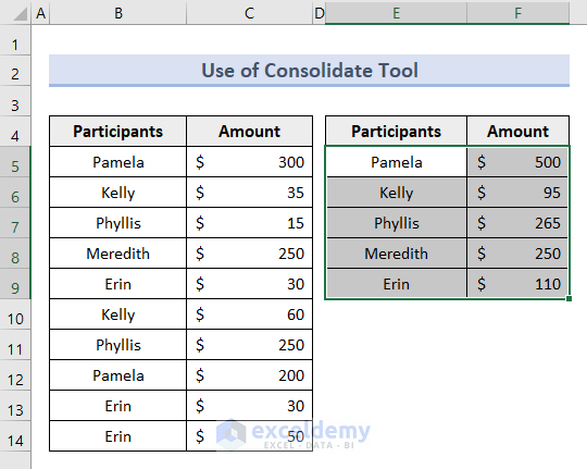
Method 9 – Summarize Data Without a Pivot Table Using the Consolidate Tool
- Go to the Data tab and select the Consolidate icon under the Data Tools group.

- The Consolidate window pops up.
- Insert the Function Sum.
- Insert the cell range B5:C9 as Reference.
- Keep the Left Column box checked.
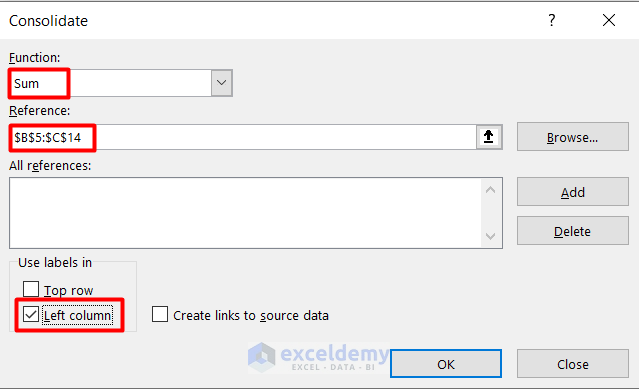
- Press OK.
- You can apply any other function as well in the Function box.
Read More: How to Summarize Data by Multiple Columns in Excel
Method 10 – Use Excel VBA to get Unique Values
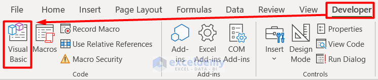
- Go to the Developer tab and select Visual Basic.
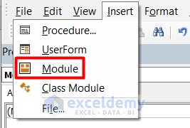
- In the new window, select Module under the Insert section.
- Insert this code on the blank page:
Sub ListDuplicates()

    For x = 1 To Cells(Rows.Count, "B").End(xlUp).Row
         If Application.WorksheetFunction.CountIf(Range("B:B"), Range("B" & x)) > 1 Then
            If Application.WorksheetFunction.CountIf(Range("E:E"), Range("B" & x)) = 0 Then
                Range("E" & Cells(Rows.Count, "E").End(xlUp).Row + 1).Value = Range("B" & x).Value
            End If
         End If
    Next x
End Sub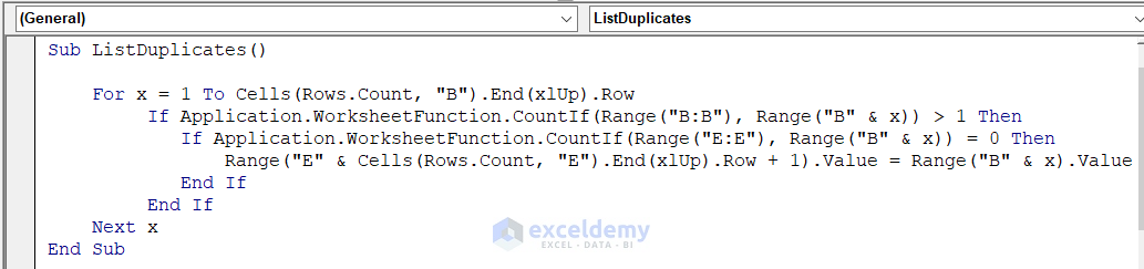
- Press F5 or click on the Run Sub button.

- Click on Run on the Macros window.
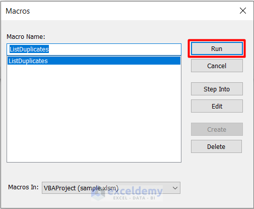
- You will get the unique names next to the dataset.
Download the Practice Workbook
Related Articles
- How to Make Summary in Excel From Different Sheets
- How to Create Summary Table from Multiple Worksheets in Excel
- How to Create Summary Table in Excel

