How to Summarize Text Data in Excel – 3 Steps

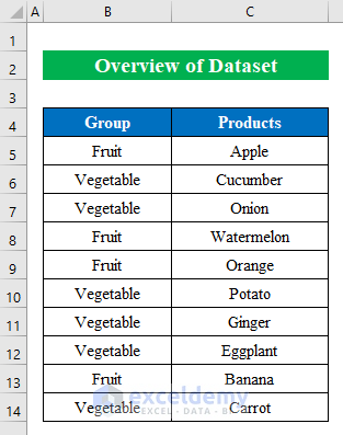
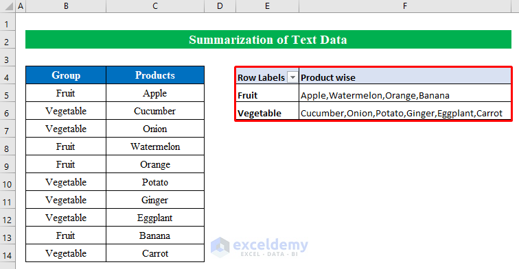
The dataset showcases Products and their Groups. To summarize all products:

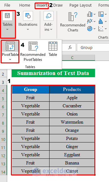
Step 1 – Create a Pivot Table

• Select the whole dataset and go to “Insert”.
• Select “Pivot Table”.

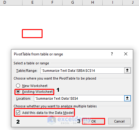
• The “PivotTable from table or range” window will be displayed.
• Select “Existing Worksheet” and choose a location in your workbook.
• Check “Add this data to the Data Model”.
• Click OK.

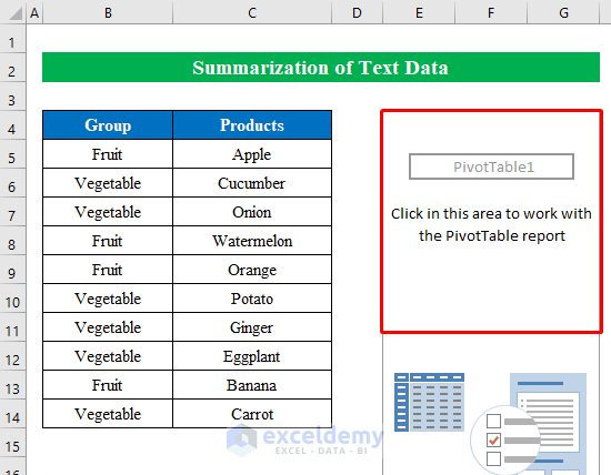
The pivot table is created in the same worksheet.

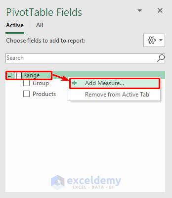
Step 2 – Apply the DAX Formula to the Selected Range

• Right-click and place the cursor over “Range”.
• Choose “Add Measure”.

• In the “Measure” window, enter a name in “Measure Name”.
• Enter the formula and click OK.

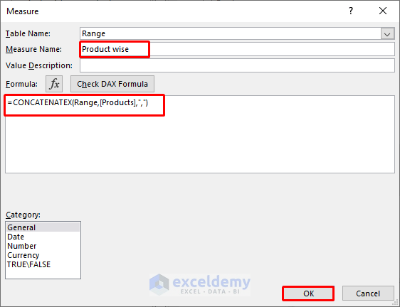
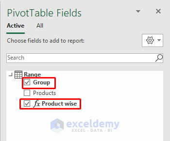
• A new field is added to the pivot table.
• Check the boxes shown below.

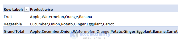
• Data is summarized in the pivot table.

Step 3 – Remove the Grand Total from Final Output

• Select any cell in the pivot table and choose “Off for Rows and Columns” in “Design”.

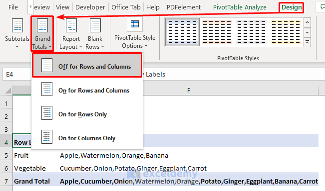
This is the output.

Read More: How to Summarize Subtotals in Excel

Things to Remember

• The VLOOKUP and SUMIF functions are used to summarize data with numeric values. To summarize text data you cannot use the VLOOKUP function.

Download Practice Workbook

Download the practice workbook.

Related Articles

• How to Summarize a List of Names in Excel
• How to Group and Summarize Data in Excel
• How to Create a Summary Sheet in Excel
• How to Make Summary in Excel From Different Sheets
• How to Summarize Data by Multiple Columns in Excel
• How to Summarize Data Without Pivot Table in Excel
• How to Create Summary Table in Excel
• How to Create Summary Table from Multiple Worksheets in Excel

<< Go Back to Summarize Data In Excel | Data Analysis with Excel | Learn Excel