How to Summarize Data in Excel (8 Easy Methods)

Download the Practice Workbook

8 Useful Methods to Summarize Data in Excel

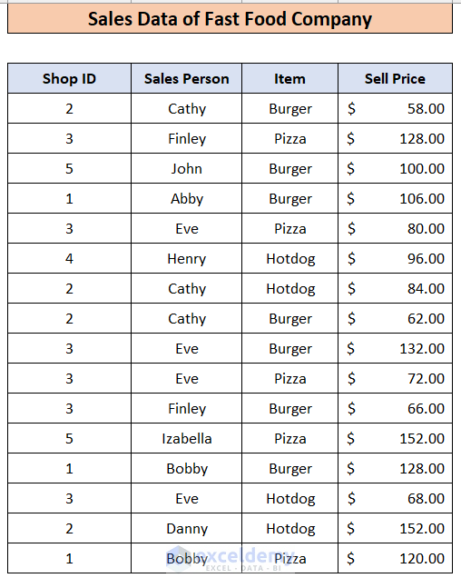
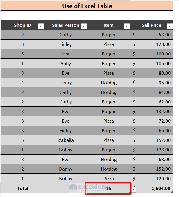
We have some sales data for a fast-food company on a particular day. This company has 5 shops in different places, each with two salespersons. Their selling items are burgers, pizza, and Hot dogs.

Method 1 – Apply the AutoSum Option to Summarize Data

Let’s calculate the total sales.

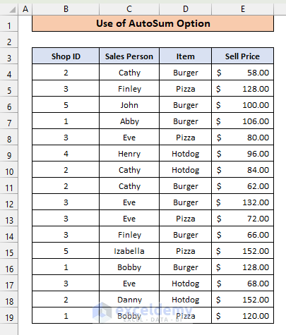
Steps:

• Click on the cell where you want to display the sum. We have selected H4.
• Click on the AutoSum icon (Greek letter Sigma) in the Editing ribbon.
• Select the cells which contain the selling price.

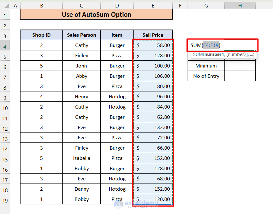
• Close the parentheses.
• Click Enter.

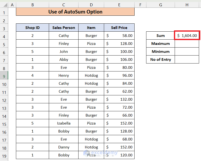
• If you click on the down arrow adjacent to the AutoSum icon, you will see 4 more options:

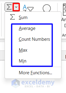
• Similar to the Sum option, you can use these functions to summarize your data.
• The Average function will give you the average value of the data.

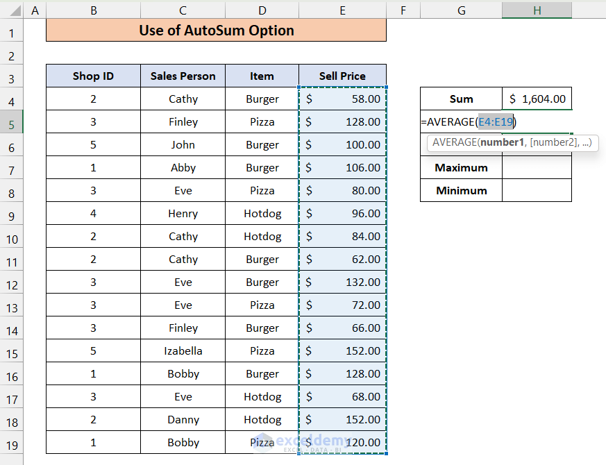
• Here’s the average data.

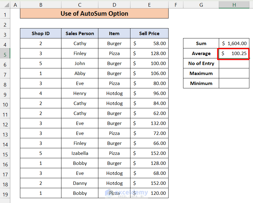
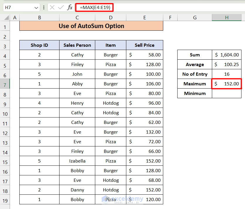
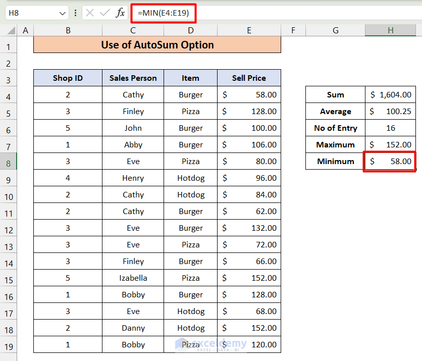
• You can calculate the number of entries, maximum, and minimum value by using the Count Numbers, Max, and Min options, respectively.
• Result of Count Numbers.

• The result of MAX.

• The result of MIN.

Method 2 – Use Excel Functions to Summarize Data

Case 2.1 – The SUM Function

Steps:

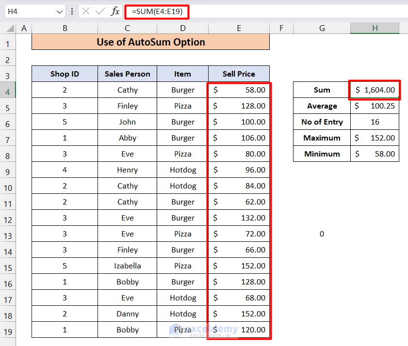
• Select cell H4.
• Insert the formula:

• Press Enter and you will get exactly the same result.

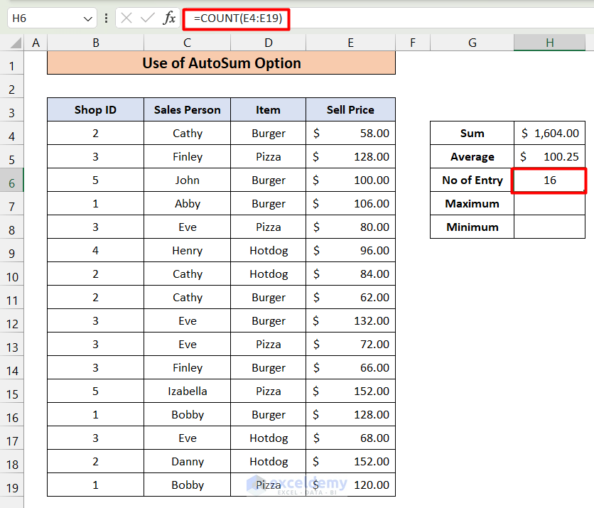
Case 2.2 – The COUNT Function

Steps:

• Select Cell H6.
• Insert the following:

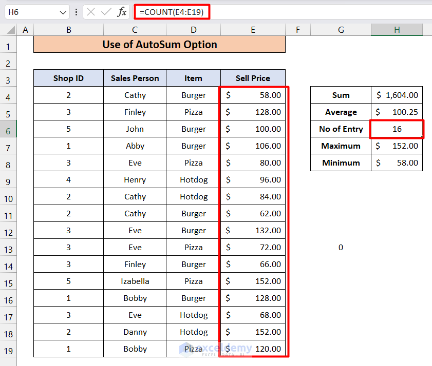
Case 2.3 – COUNTA Function

We can only apply the COUNT function to the cells containing numeric values. COUNTA counts all values.

Steps:

• If we use the COUNTA function for cells D4 to D19, we’ll get the same answer.

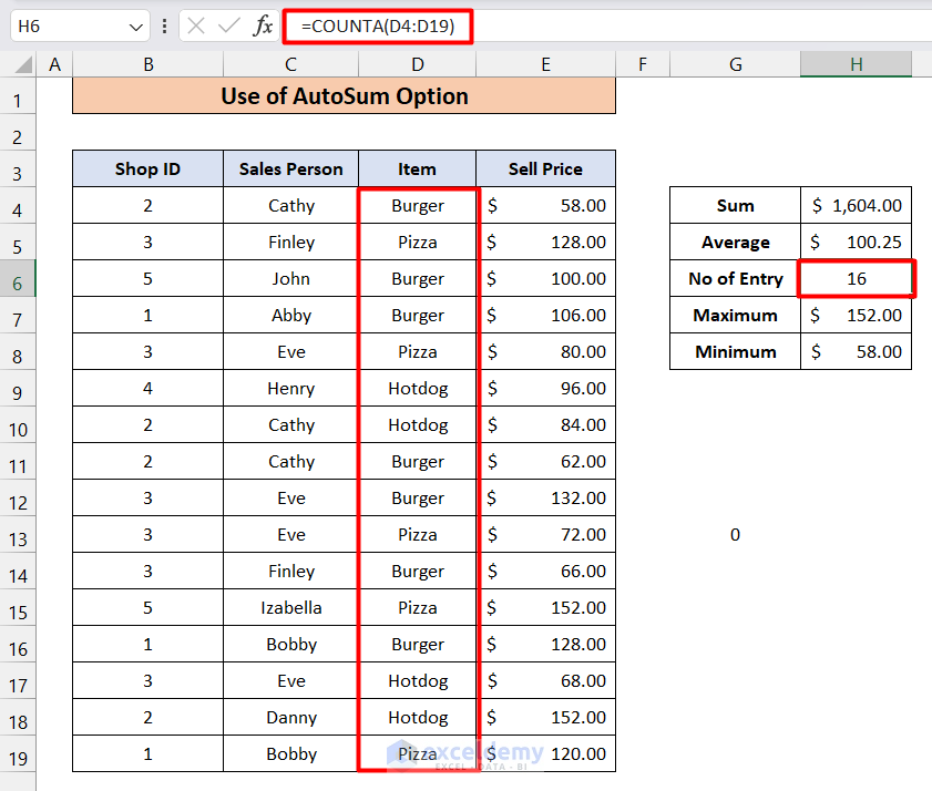
Case 2.4 – The AVERAGE Function

Steps: 

• In cell H5, apply the AVERAGE function:

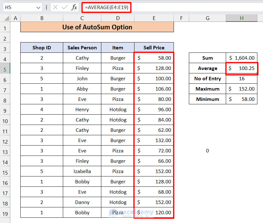
Case 2.5 – The SUMIF Function

Steps:

• We want to see the sales of Burger only.
• Apply the following formula:

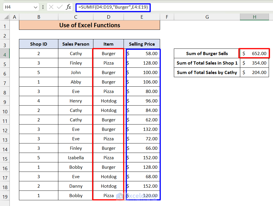
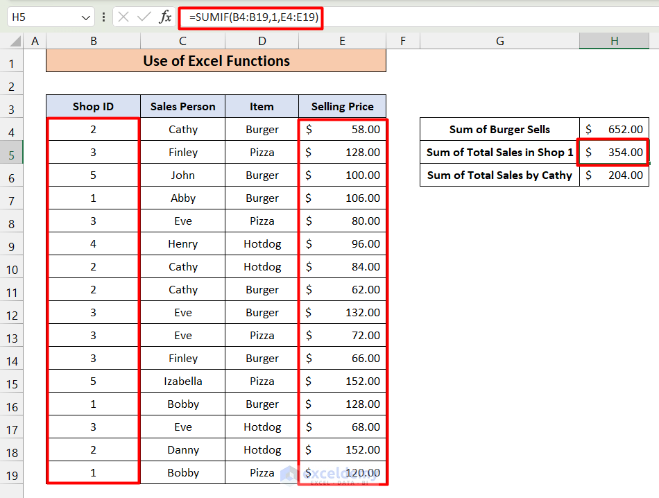
• We can also calculate the total sales in shop 1 by applying the following formula:

• Here is the result.

• The formula for calculating the total sales made by Cathy:

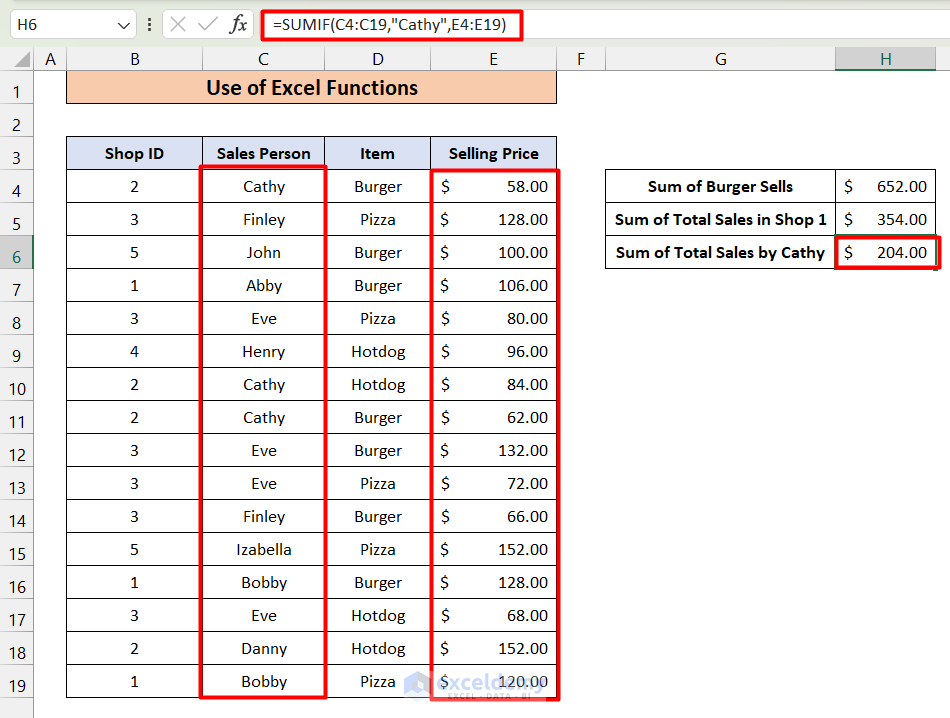
Case 2.6 – The SUMIFS Function

If we want to sum with more criteria, we have to use the SUMIFS function.

Steps:

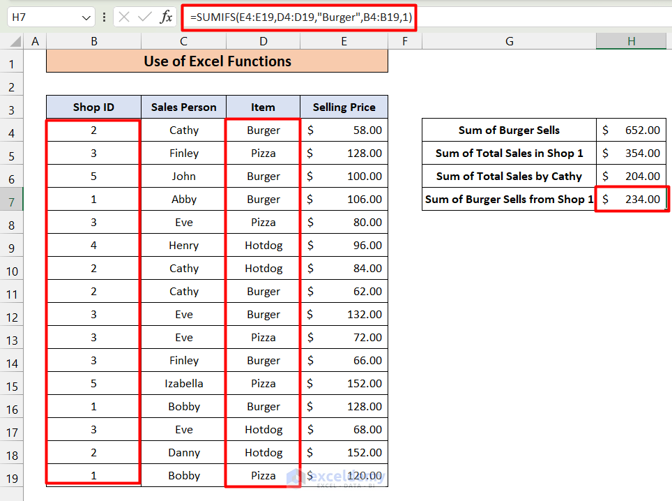
• We want to know the number of sales for Burger from Shop 1.
• Apply the following formula.

• Hit Enter and you will get the following result.

Case 2.7 – The COUNTIF Function

We can use the COUNTIF function to calculate the number of entries for a certain condition.

Steps:

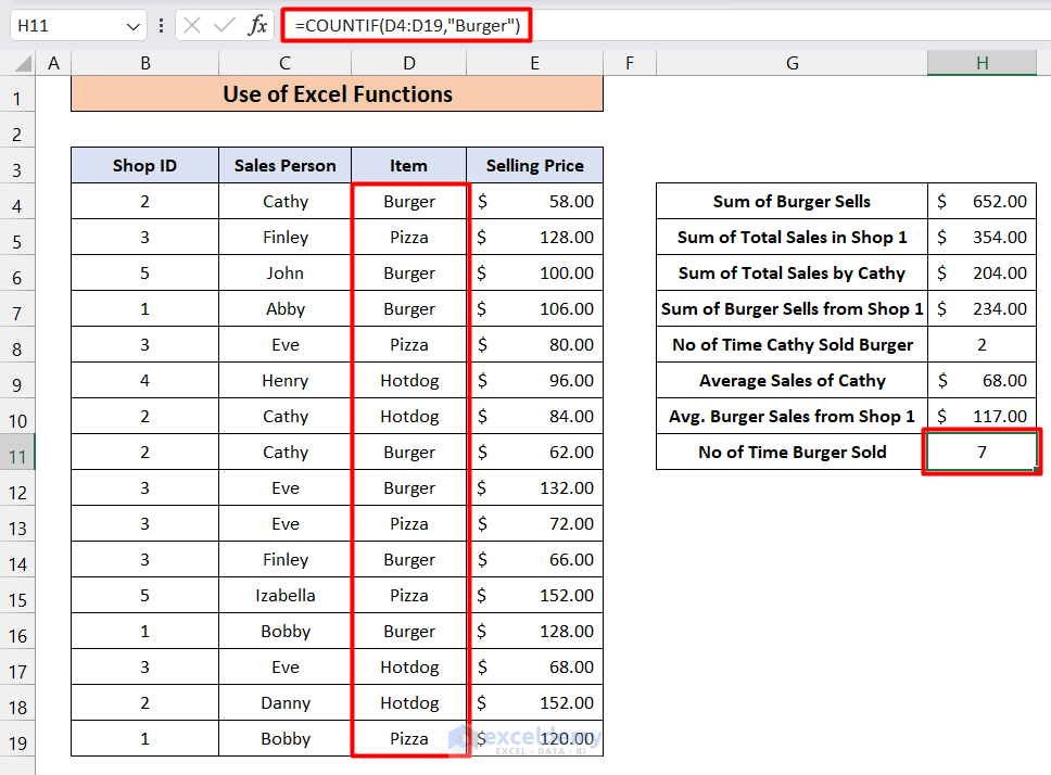
• We want to calculate the number of orders with burgers across 3 shops. Use the following formula:

D4:D19 is the Item range where the number of cells that meet the criterion will be counted. “Burger” is the criterion that is to be satisfied in the range D4:D19.

• Press Enter and you should see the following result.

Case 2.8 – The COUNTIFS Function

We use the COUNTIFS function when counting on multiple conditions.

Steps:

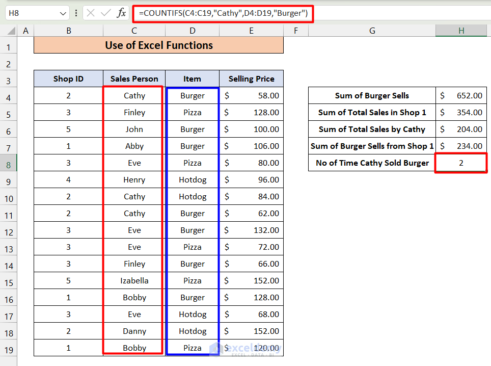
• If we want to find out how many times Cathy sold Burgers, we can use the following formula:

• Press Enter and you should get the following result.

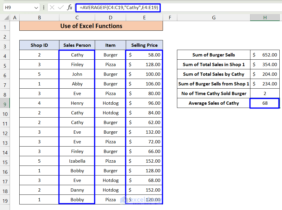
Case 2.9 – The AVERAGEIF Function

Steps:

• Here’s how to calculate the average value of sales for Cathy:

• You should get the following result.

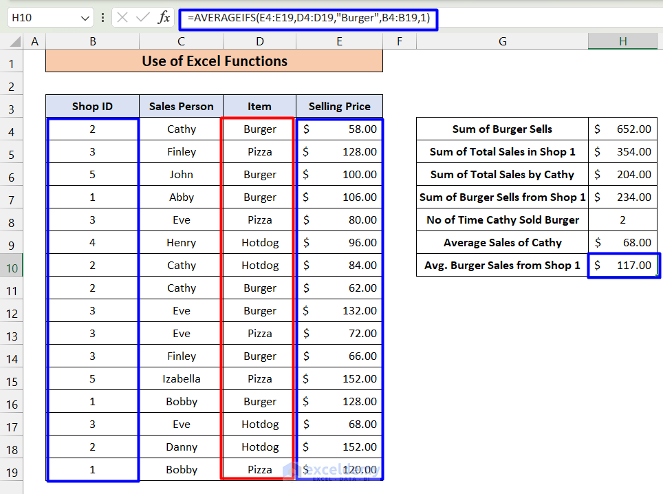
Case 2.10 – The AVERAGEIFS Function

Steps:

• To calculate the average amount of sales of Burger from shop 1, use the following formula:

• Hit Enter and you will get the following result.

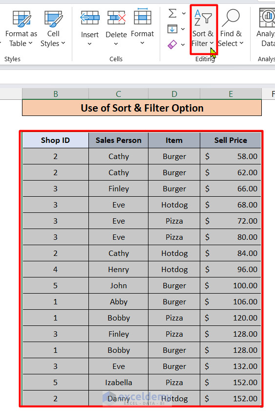
Method 3 – Apply the Sort & Filter Option to Summarize Data

• Go to the Sort & Filter option in the Editing ribbon to get more filter options.

• You can make the order from A to Z, from Z to A, or apply Custom Sort. The first two options sort the data based on the first column. If you want to do sorting based on other columns, you have to choose the Custom Sort option. We’ll sort the data based on the Item column.

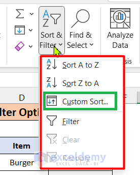
• Click on Custom Sort and you’ll see a window like this.

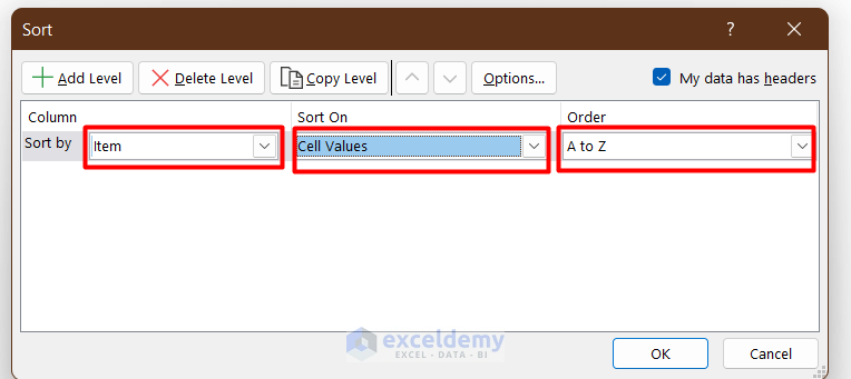
• From the Column drop-down list, select Item.
• From Sort On the drop-down list, select Cell Values.
• From the Order drop-down list, select A to Z.
• Click OK.

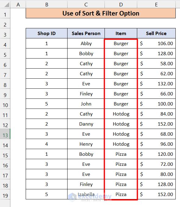
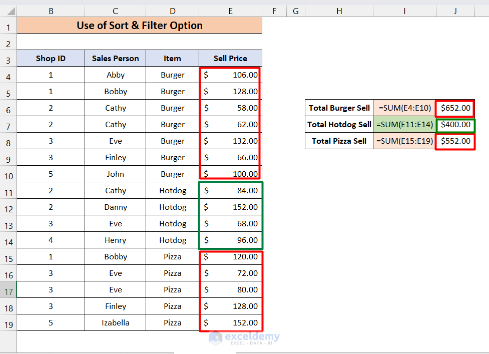
• We can perform many calculations easily as we have the data sorted. We will find the total burger, pizza, and hot dog sales.

• You can also play with other custom filter options and see which one is the most appropriate for you.
• If you choose Filter, you will see an icon on each column header like below:

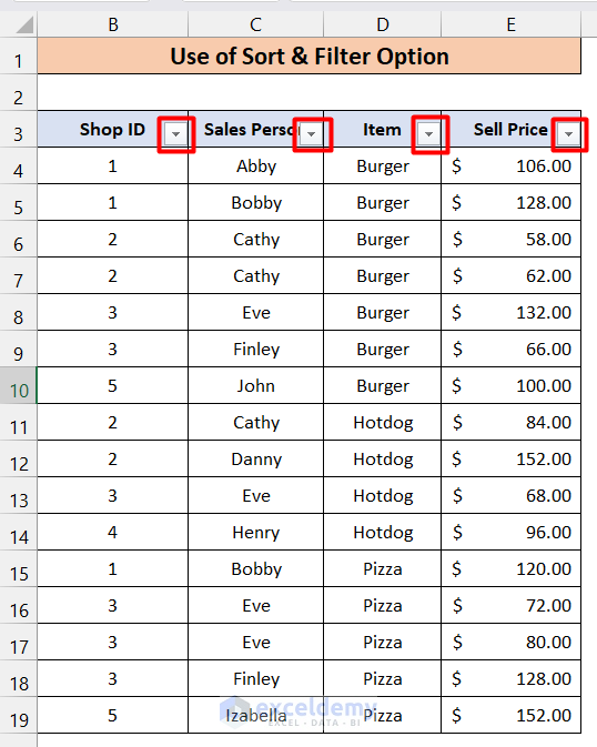
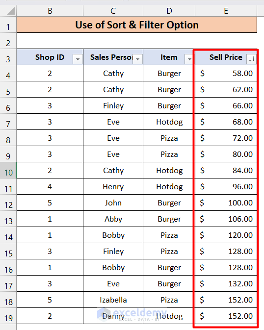
• By clicking on any of the icons, you can sort the data according to the values in that column. We have sorted our data based on Sell Prices from smallest to largest.

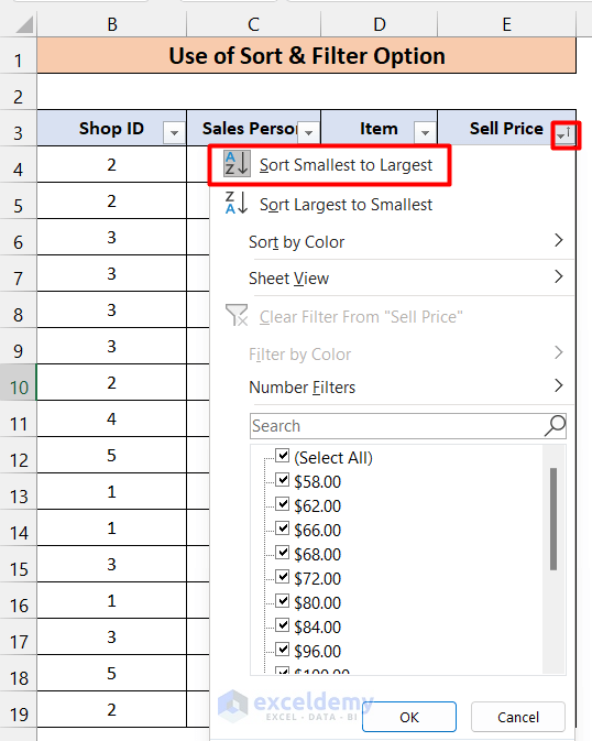
• Here is the result.

Method 4 – Perform the Subtotal Command to Summarize Data

Steps:

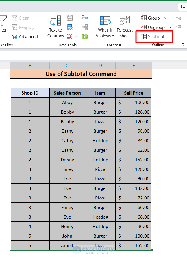
• Select the data and go to the Data tab.

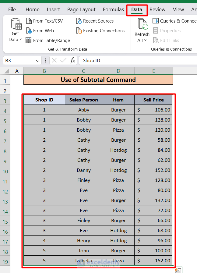
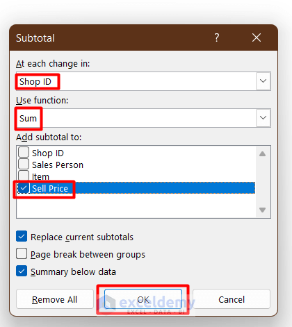
• Click on Subtotal in the Outline group.

• You will see a pop-up like this.
• Check the options as in the image and click OK.

• You will see the following results.

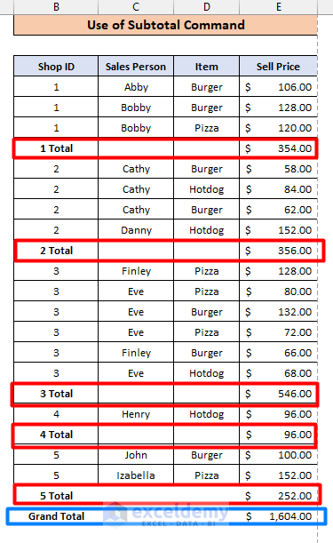
• You can also find the average, maximum, and minimum values of each subgroup. Visit our website to learn more about the Subtotal option.

Method 5 – Create an Excel Table to Summarize Data

Steps:

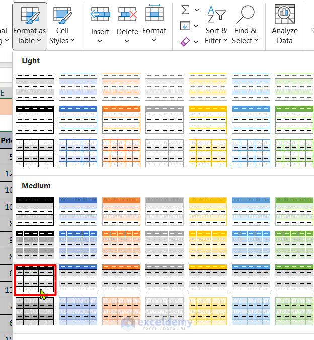
• Select all the cells and select the Format as Table option from the Styles ribbon.

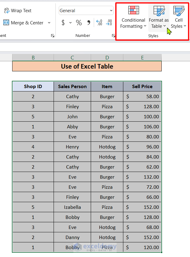
• Choose any suitable design from below.

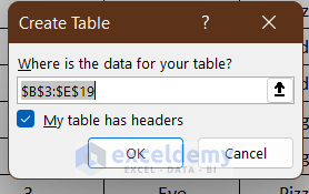
• A window will pop up like this. Check the box and click OK

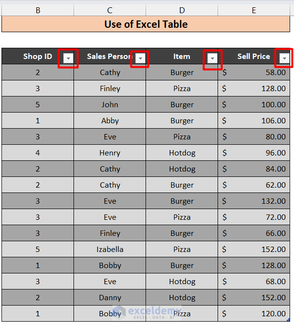
• You will get a table. It has the filter in the header columns like the Sort & Filter method.

• Go to the Table Design tab and check Total Row.

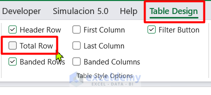
• A row will be added below the table with totals.

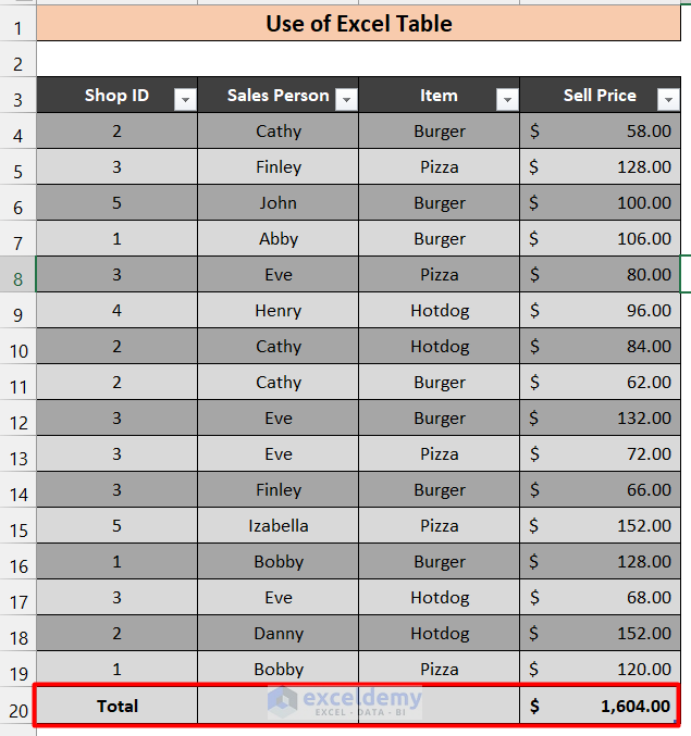
• We have calculated in the Sell Price column. Each cell in the row will have a dropdown menu containing multiple functions.

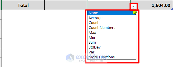
• You can use those functions to directly calculate the value you want. If we want to calculate the number of entries, we have to select the Count option.

Method 6 – Utilize the Slicer Feature in an Excel Table for Summarizing Data

Steps:

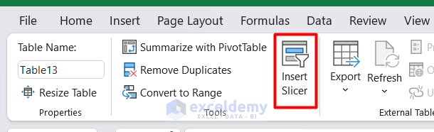
• Go to the Table Design tab and select the Insert Slicer option.

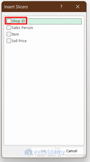
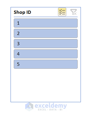
• Check Shop ID and click OK.

• You will see another window with buttons.
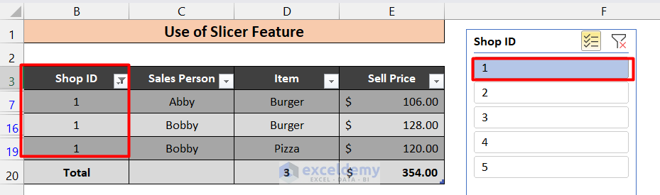
• Select any Shop ID and the table will show the data only related to this shop. We have shown this for Shops 1 and 2.

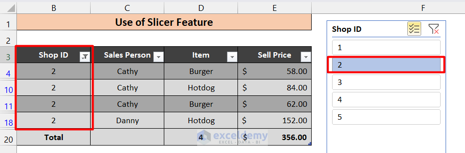
• Here’s the filter for Shop 2.

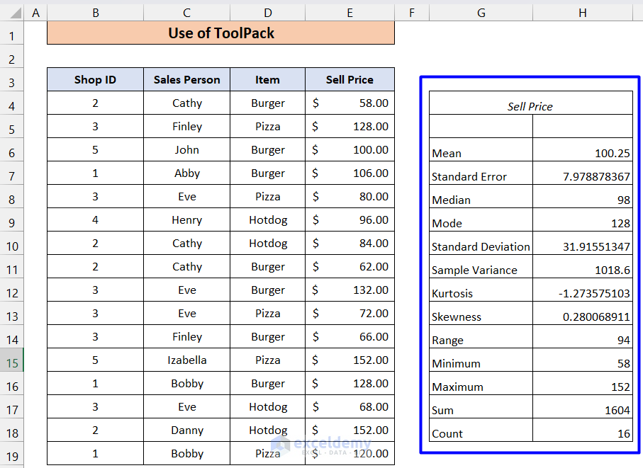
Method 7 – Run the Data Analysis ToolPak to Summarize Data

Steps:

• Go to the File tab, then click on Options.

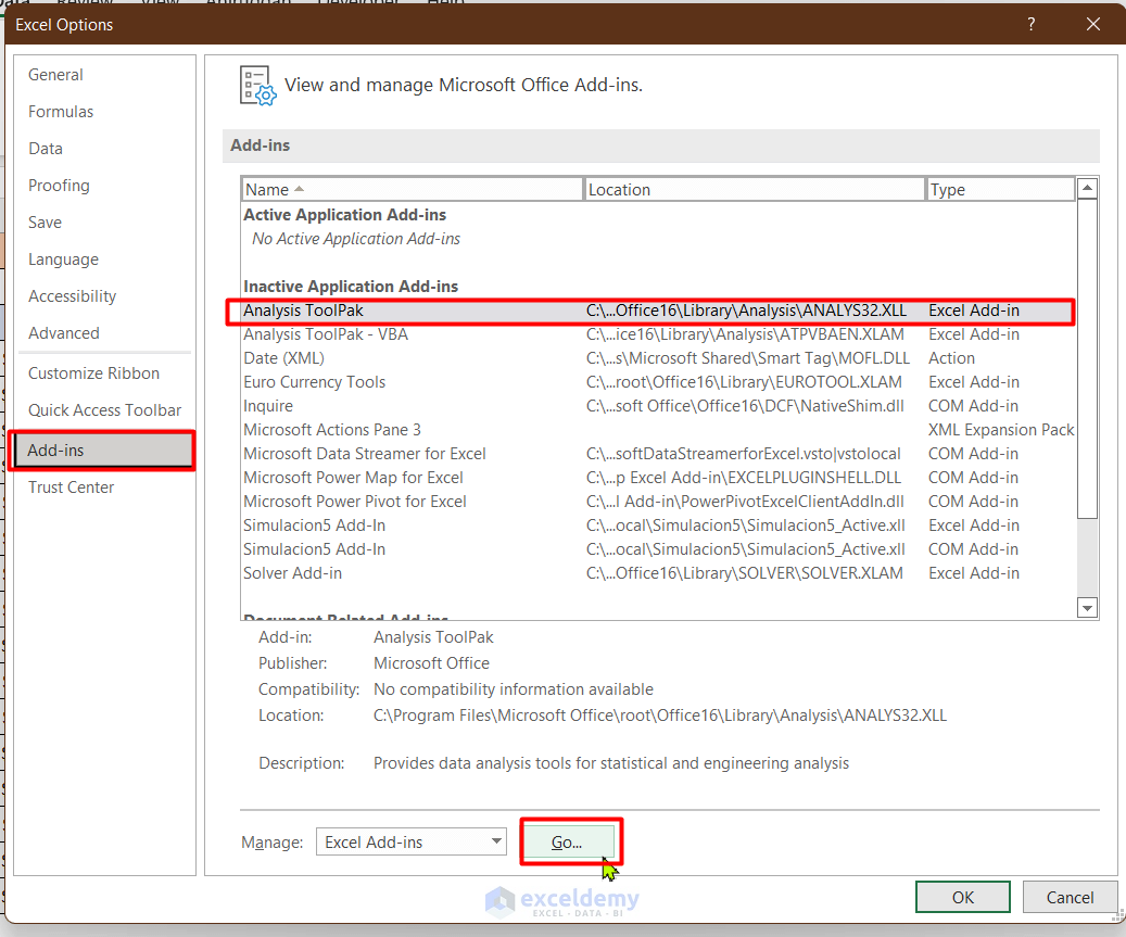
• Go to Add-ins, select Analysis ToolPak, and click on Go. A new window will pop up.

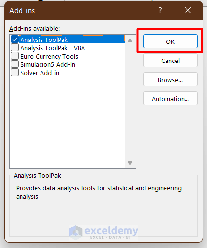
• Check on the Analysis ToolPak and click OK. This will enable the Data analysis tool on the Data Tab which you will find in the top-right corner.

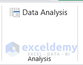
• Click on Data Analysis. A dialog box like this will open up.

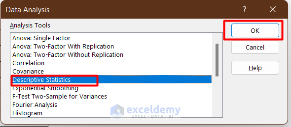
• Click on Descriptive Statistics and click OK. A new window will pop up.

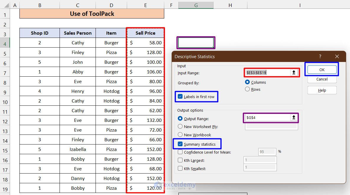
• Input the as shown in the figure with color boxes. In the input range, select the column that contains numeric values. We have selected the Sell Price column.
• In the Output Range, select the cell where you want to place your Summary statistics. We have selected G4.
• Check the Labels in the first row and Summary statistics.
• Click OK. You will get the result as follows.

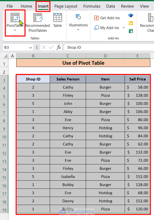
Method 8 – Use a Pivot Table to Summarize Data

Steps:

• Select the data cells and go to Insert tab.
• Click on PivotTable.

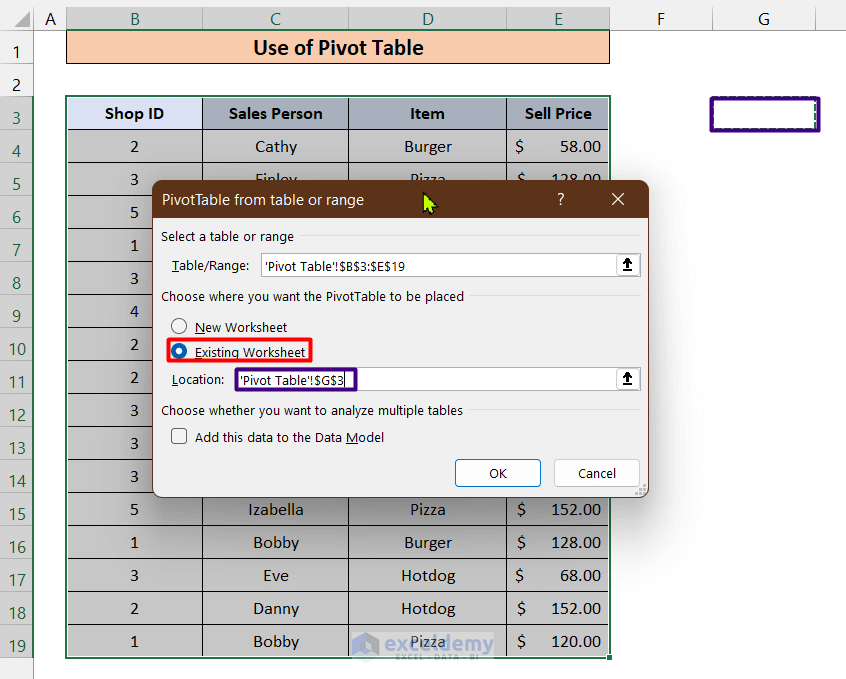
• Click on Existing Worksheet and choose a suitable cell to place the pivot table.
• Click OK.

• This generates a new table.

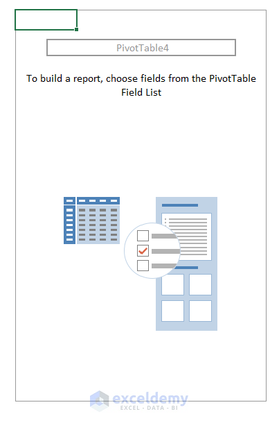
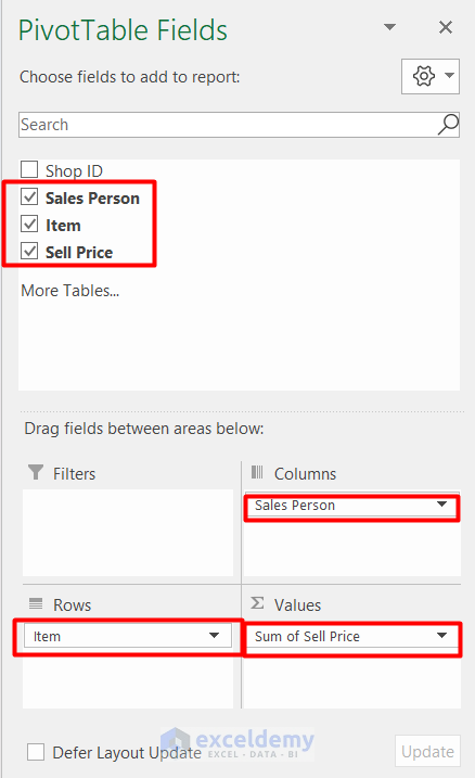
• On the right side, you will see PivotTable Fields.

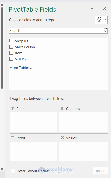
• Drag and drop the ranges in the corresponding fields like below.

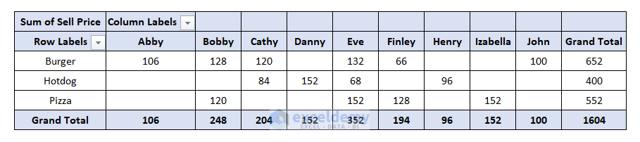
• We have created a table which contains your desired summary of data.

Things to Remember

• You should use the first method if your data is considerably small in quantity as it is the quickest one.
• If you have a large quantity of data, use the Pivot table method
• You should only use the Data Analysis Toolpack if you need in-depth statistical analysis like Skewness, Kurtosis, etc.

Summarize Data in Excel: Knowledge Hub

• How to Summarize Text Data in Excel
• How to Summarize Data by Multiple Columns in Excel
• How to Summarize Data Without Pivot Table in Excel
• How to Create Summary Table in Excel
• How to Create Summary Table from Multiple Worksheets in Excel
• How to Summarize Subtotals in Excel
• How to Summarize a List of Names in Excel
• How to Group and Summarize Data in Excel
• How to Create a Summary Sheet in Excel
• How to Make Summary in Excel From Different Sheets

<< Go Back to Data Analysis with Excel | Learn Excel