Organize Data in Excel: A Complete Guide

We often need to organize data in Excel while working for easy data management, better data analysis, better visualization, and more efficiency. Here’s an overview of how you can easily sort data.

Overview image of Organize data in Excel

Download the Practice Workbook

Organize Data in Excel.xlsx

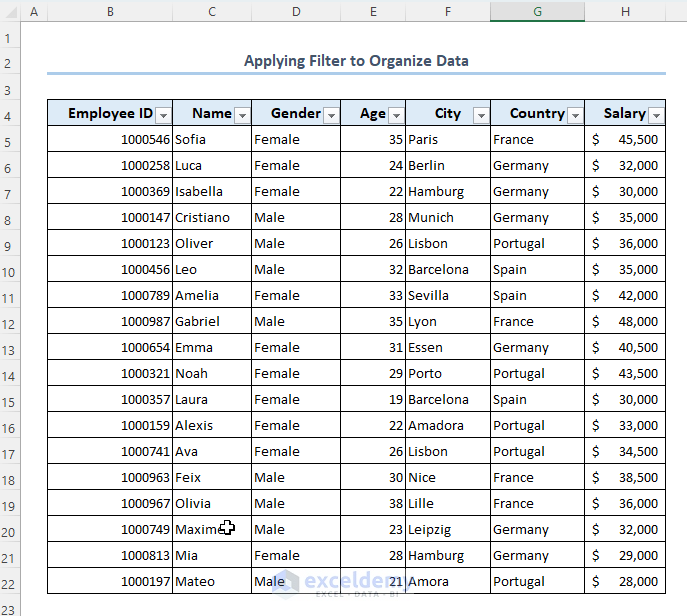
How to Organize Data in Excel

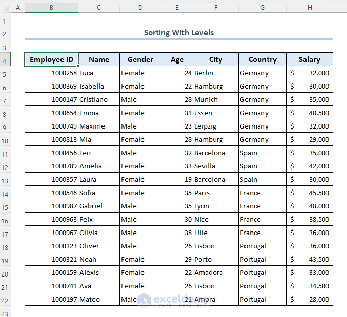
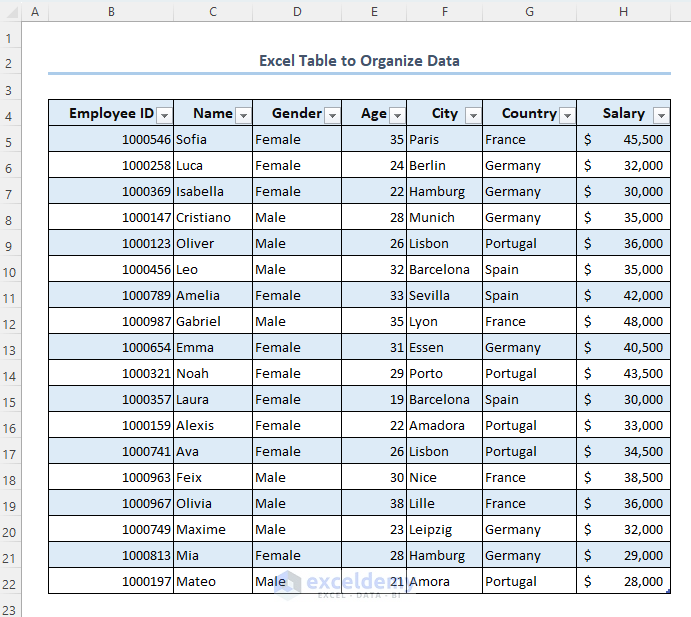
We will be using the following dataset to describe how to organize data in Excel, which uses employee information.

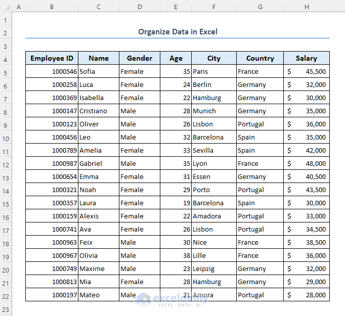
Method 1 – Organize Data by Using the Sort Feature

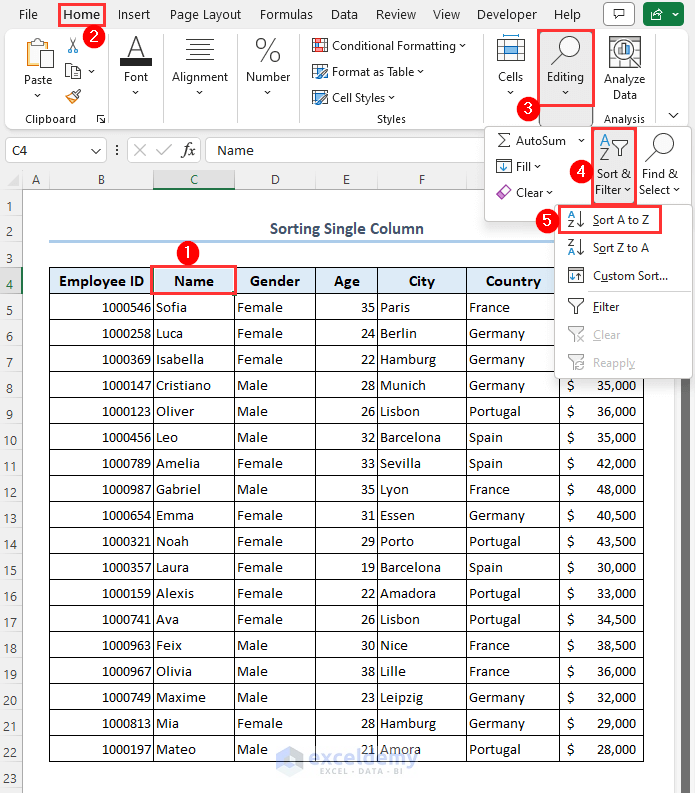
Case 1.1 – Sorting a Single Column

Let’s sort the employee names alphabetically A to Z.

Click on column header Name.
Go to Home, then to Editing.
Click on Sort & Filter and select Sort A to Z.

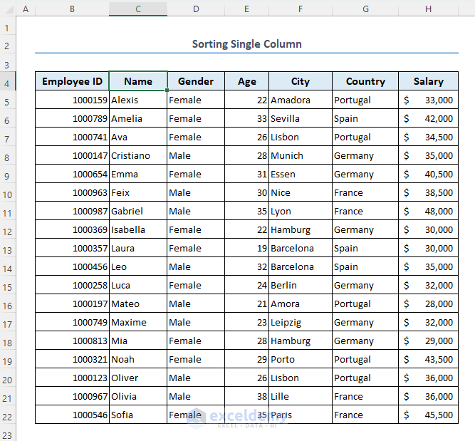
You can see that the names of all the employees are arranged in alphabetical order.

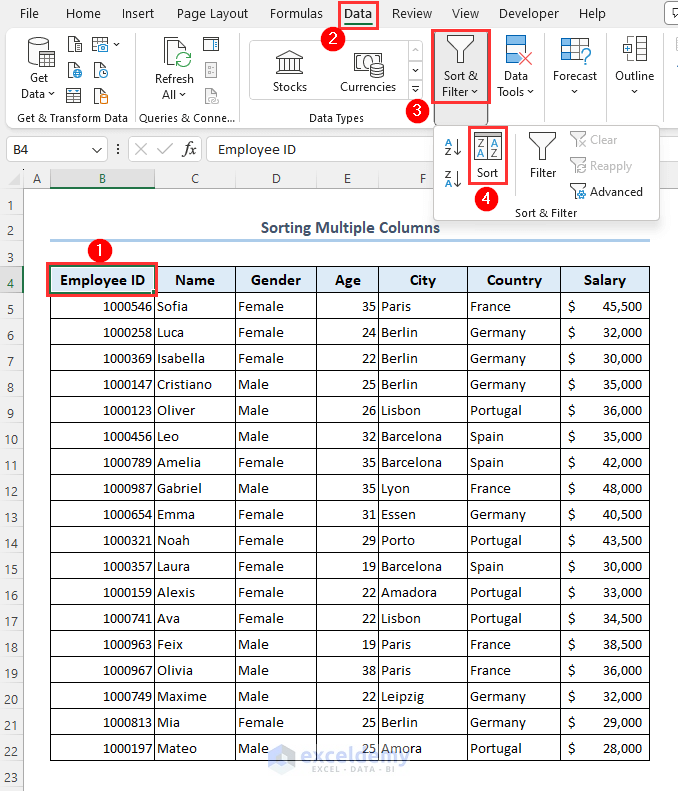
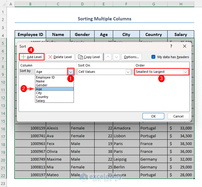
Case 1.2 – Sorting Multiple Columns

Let’s arrange the data by age, then by city, then by name.

Select anywhere in your dataset.
Go to Data, then choose Sort & Filter and select Sort.

A dialog box Sort will appear.
In the Column section, click on the Sort by drop-down menu then select Age.
Select Smallest to Largest from the Order group.
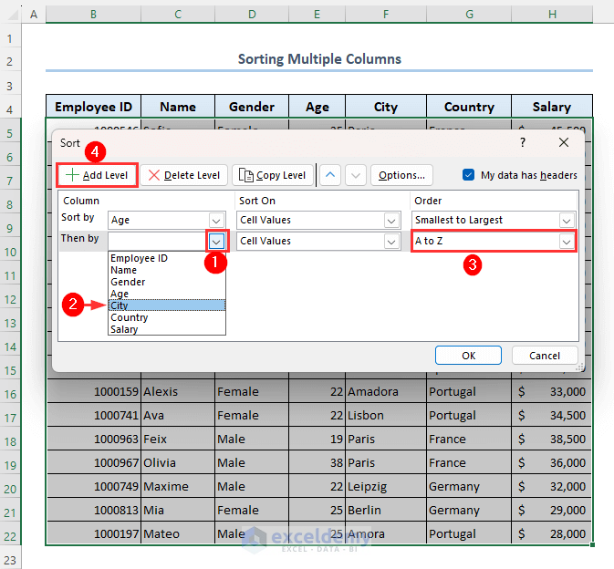
Click on Add Level.

Select City from the Then by drop-down.
Select A to Z from the Order column as shown.
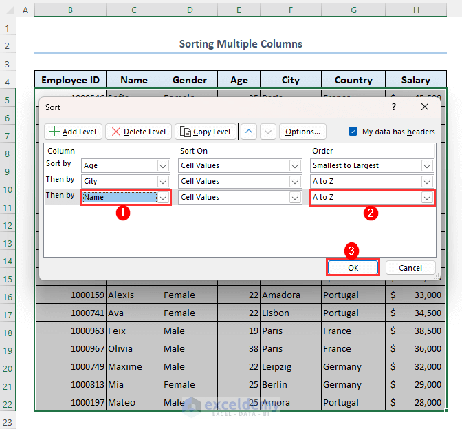
Click on Add Level again.

Select Name from the Column section.
Select A to Z from the Order group.
Click on OK.

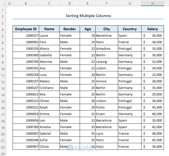
The final output will be as follows.

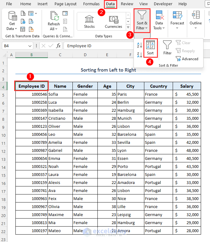
Case 1.3 – Sorting from Left to Right

Select cell B4 which is the Employee ID header.
Go to the Data tab.
Click on the Sort & Filter menu.
Select Sort.

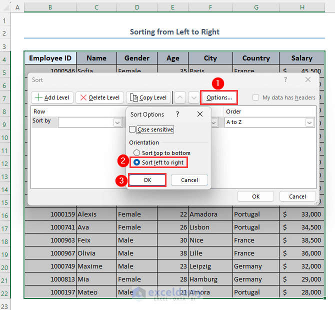
From the Sort dialog box, click on Options.
The Sort Options dialog box will appear. Select the Sort left to right option.
Click on OK.

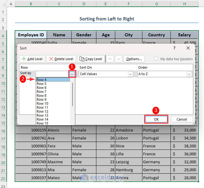
From the Row section in the Sort by drop-down menu, select Row 4 as our dataset starts from row 4.
Select the order you want from the Order column. We have selected A to Z.
Click on OK.

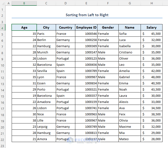
Data will be sorted from left to right.

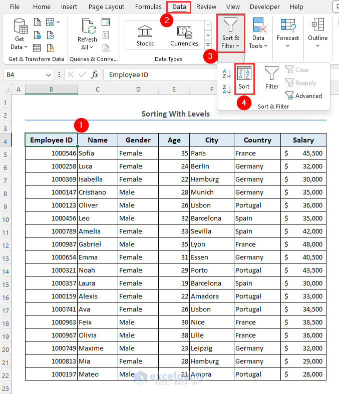
Case 1.4 – Sorting with Levels

Let’s arrange your data by sorting those with levels. Let’s arrange those employees in the following order: Germany, Spain, France, Portugal.

Select your dataset.
Go to the Data tab.
Click on the Sort & Filter option.
Select Sort.

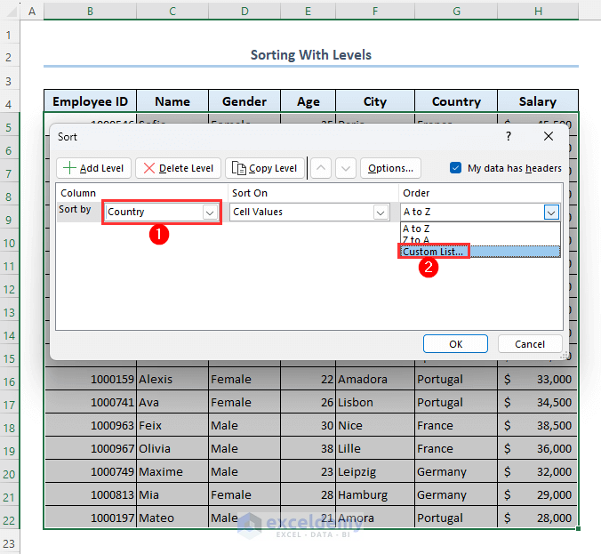
Select Country from the Column section.
From the Order column, select Custom List.

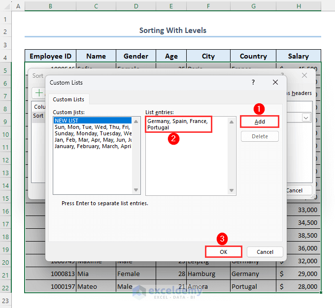
Type Germany, Spain, France, Portugal in the List entries box.
Click on Add.
Click on OK.

Click on OK again.

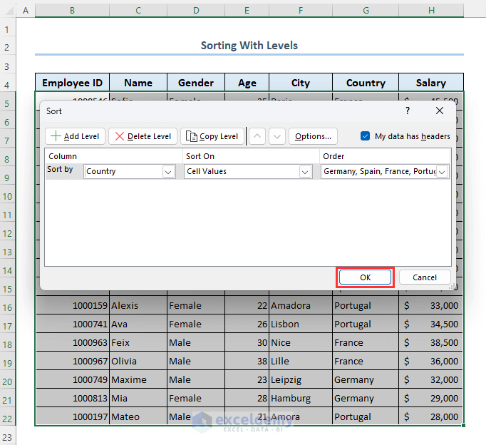
Your dataset will be organized as follows.

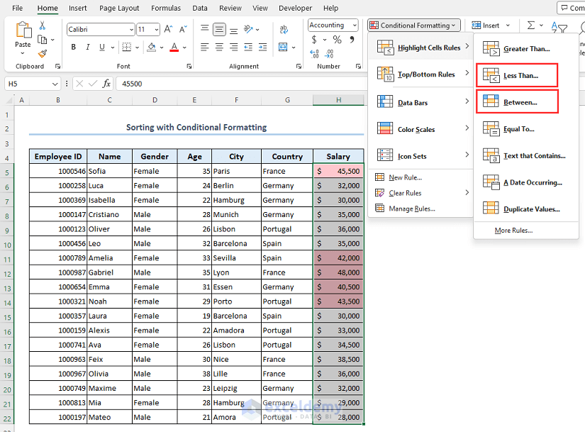
Case 1.5 – Sorting with Conditional Formatting

Let’s highlight salaries which are greater than $40,000 with a Light Red color.

Select the range H5:H22.
Go to Conditional Formatting then select Highlight Cells Rules and choose Greater Than.

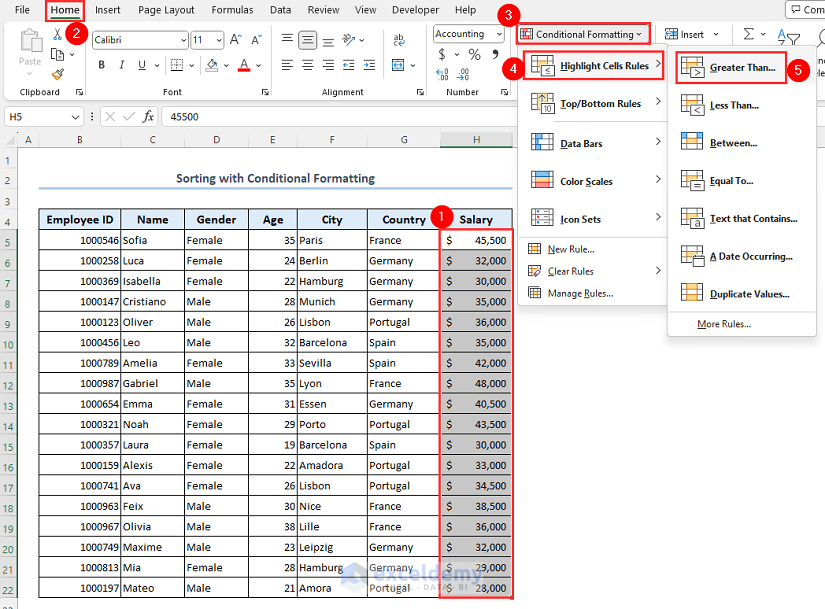
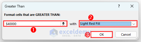
A dialog box titled Greater Than will appear. Input 40000 and select a color format that you want. We have selected Light Red Fill.
Click on OK.

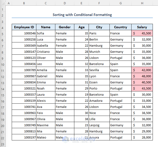
The cells which have values greater than 40,000 are highlighted as follows.

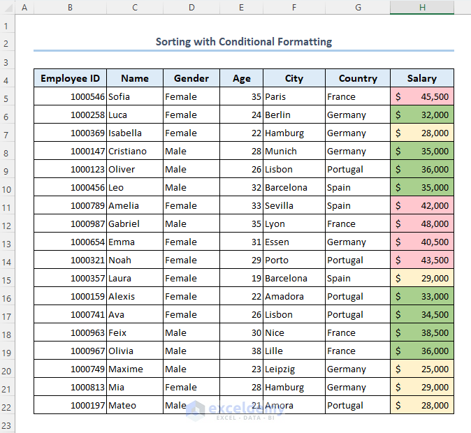
If you want to highlight salaries less than $30,000 with Light Yellow color and salaries that are between $30,000 and $40,000 with Green, use the Less Than and Between options from the Conditional Formatting menu.

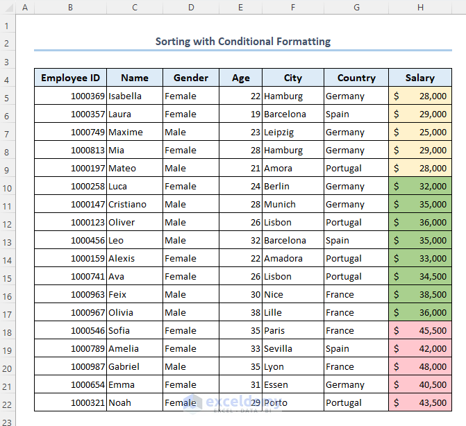
Our dataset will look like below.

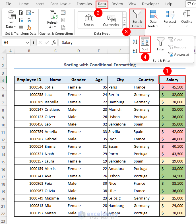
Let’s arrange the dataset based on the formatting colors: Light Yellow, Green, Light Red.
Select the dataset.
Go to Data and select Sort & Filter, then choose Sort.

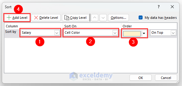
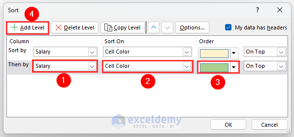
Select Salary from the Column section.
Select Cell Color from the Sort On group.
Select Light Yellow color from the Order section.
Click on Add Level.

Select Salary from the Column section as shown below.
Select Cell Color and Green color.
Click on Add Level.

Select Salary, Cell Color and Light Red color.
Click on OK.

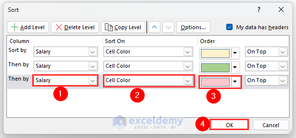
The data is organized.

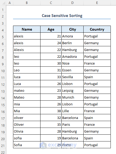
Case 1.6 – Case-Sensitive Sorting

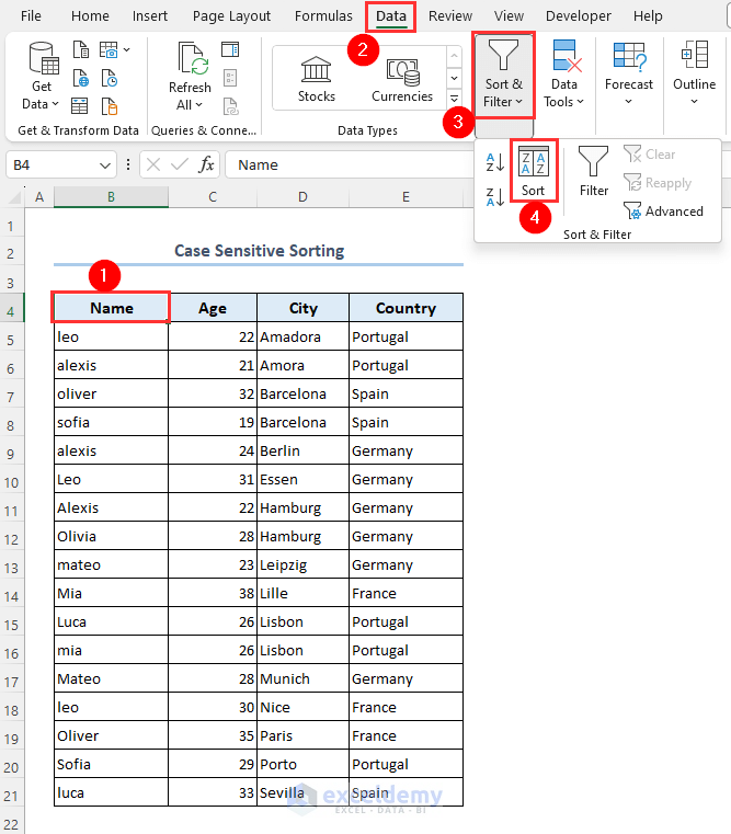
Let’s assume there are names that start with both lowercase and uppercase letters. You want to sort your data by case.

Select your dataset.
Go to Data and choose Sort & Filter, then select Sort.

A dialog box titled Sort will appear.
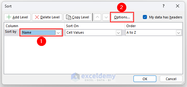
Select Name from the Column group.
Click on Options.

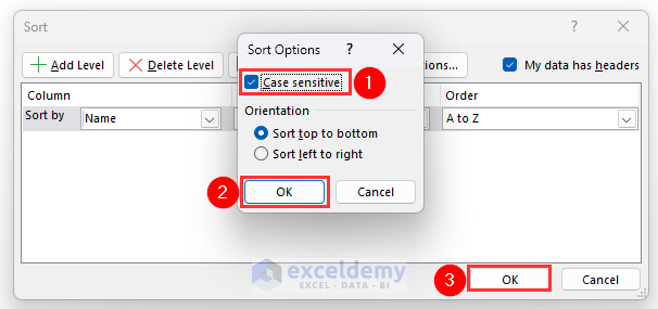
Mark the Case sensitive box.
Click on OK twice.

Your data is sorted by case as follows.

Method 2 – Apply a Filter to Organize Data

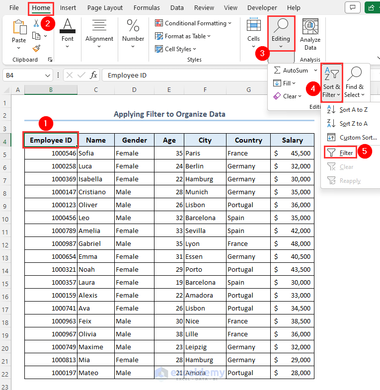
Select any header of your dataset.
Go to Home and Editing, then select Sort & Filter and choose Filter.

You can use the filters as needed.

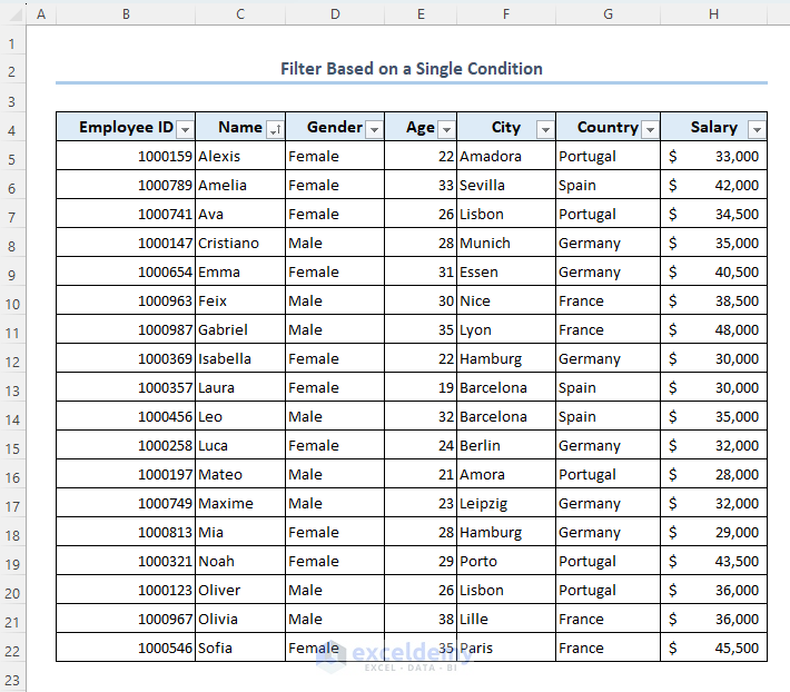
Case 2.1 – Filter Based on a Single Condition

Let’s arrange the employee names alphabetically A to Z.

Click on the arrow down icon beside the Name header.
Select Sort A to Z.

You can see that the names of all the employees are arranged in alphabetical order.

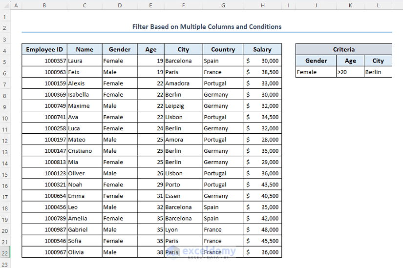
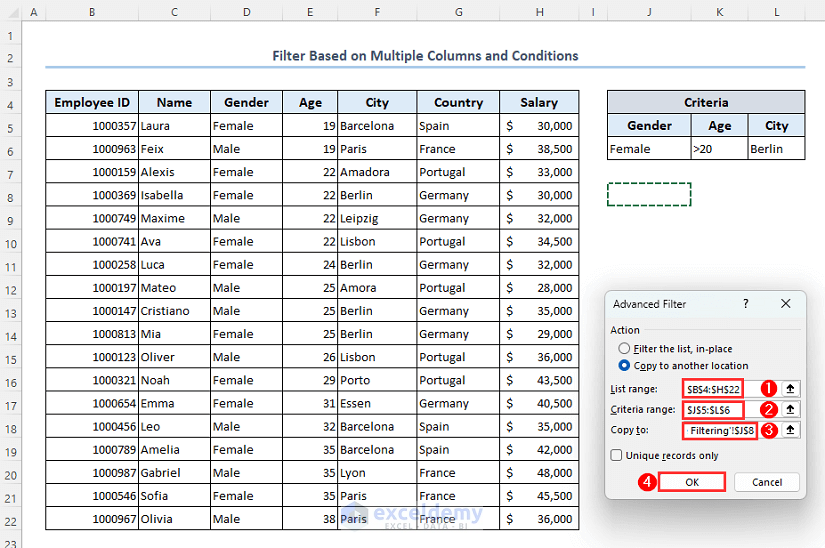
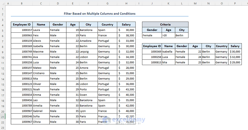
Case 2.2 – Filter Based on Multiple Columns and Conditions

Let’s show the female employees from Germany with ages greater than 20. The criteria are in a separate table to the right.

Go to the Data tab.
Click on the Advanced option.

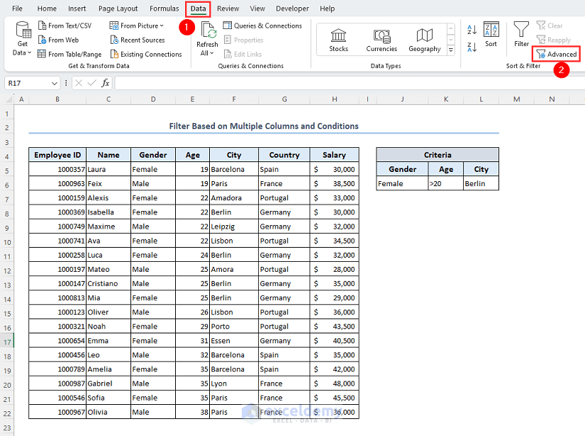
A dialog box titled Advanced Filter will appear on your worksheet.
Mark Copy to another location.
Select range B4:H22 in the List range box.
Put the range J5:L6 in the Criteria range box.
Select cell J8 in the Copy to box.
Click on OK.

Here are the results.

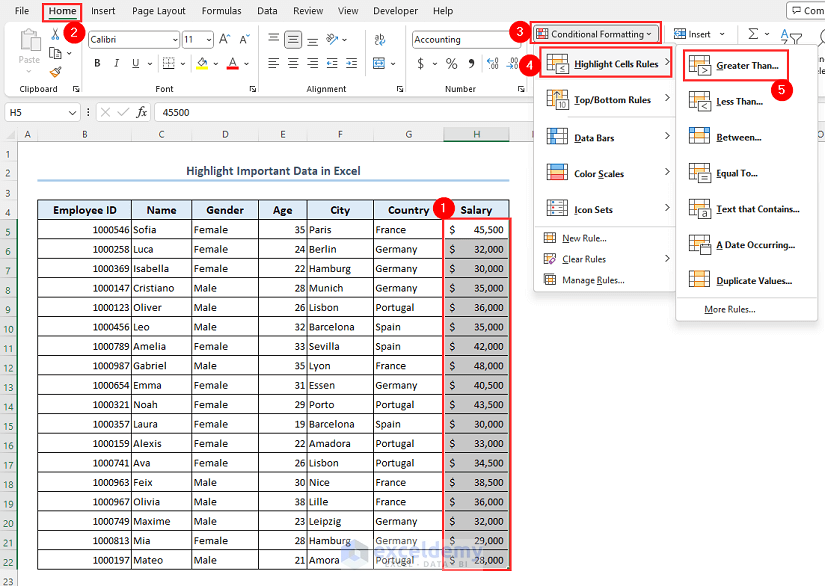
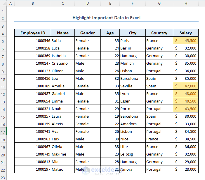
Method 3 – Highlight Important Data in Excel

Let’s highlight those salaries which are greater than $40,000.

Select the range H5:H22.
Go to Conditional Formatting, then select Highlight Cells Rules and choose Greater Than.

Insert 40000 in the first box and select any color to highlight the match cells.
Click on OK.

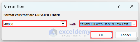
The cells are highlighted as follows.

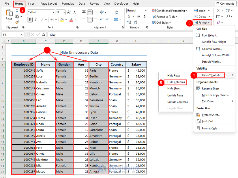
Method 4 – Hide Unnecessary Data

Let’s hide the Employee ID, Gender, and City columns from your dataset.

Select all 3 columns.
Go to Home and Format, then select Hide & Unhide and choose Hide Columns.

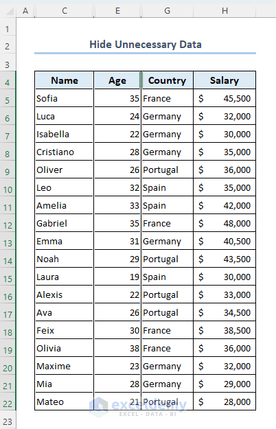
You can see that those columns are now hidden from your dataset.

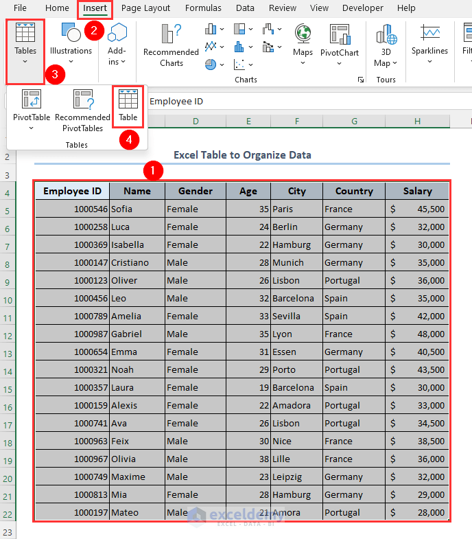
Method 5 – Use an Excel Table to Organize Data

Select the range B4:H22.
Go to Tables and select Table.

Mark My table has headers.
Cllick on OK.

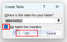
The table is created as follows. The Filter feature is added to your table as well.

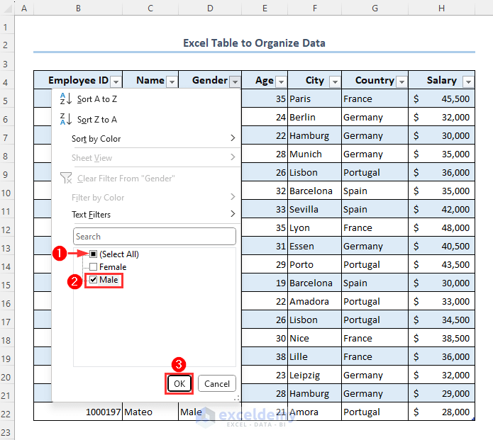
Let’s assume you want only male employees’ information.
Click on the arrow down icon beside the Gender header.
Uncheck the Select All box.
Check the Male option.
Click on OK.

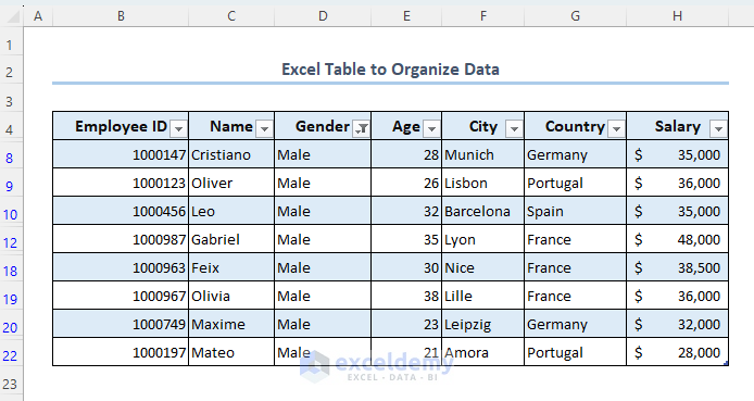
The dataset is filtered as follows.

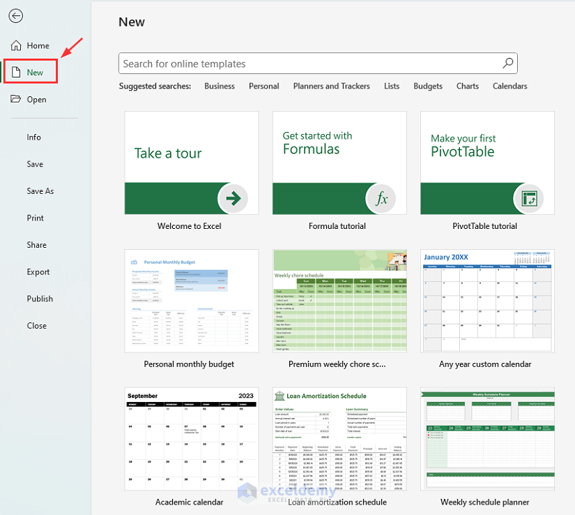
Method 6 – Organize Data Using Templates in Excel

Go to the File tab.

Click on New.
You will find several templates. You can even search for various types of templates and download them to use.

Read More: How to Organize Raw Data in Excel

Frequently Asked Questions

What is the best way to organize data in Excel?

The best way to organize data in Excel depends on the pattern of your data and how you want it to be.

What are the benefits of organizing data in Excel?

When dealing with larger datasets, organized data enables quicker decision-making and analysis.

Is it possible to create tables in Excel to organize and analyze data?

You can create a table out of a range of data in Excel by using the Table feature. It supports automatic formatting, simple sorting, and filtering, built-in calculations, etc. You can effectively manage and organize your data using tables, which makes it simpler to evaluate and work with large datasets.

Organize Data in Excel: Knowledge Hub

<< Go Back to Data Analysis with Excel | Learn Excel

Get FREE Advanced Excel Exercises with Solutions!