How to Organize Time in Excel (5 Easy Ways)

If you are searching for ways of how to organize time in Excel, this is the right place for you. Sometimes, we have to organize the dataset according to time. To organize time in Excel we can sort or create pivot tables to summarise the data. In those cases, we have to follow some simple steps. Here, in this article, you will find step-by-step ways of how to organize time in Excel.

Download Practice Workbook

5 Ways to Organize Time in Excel

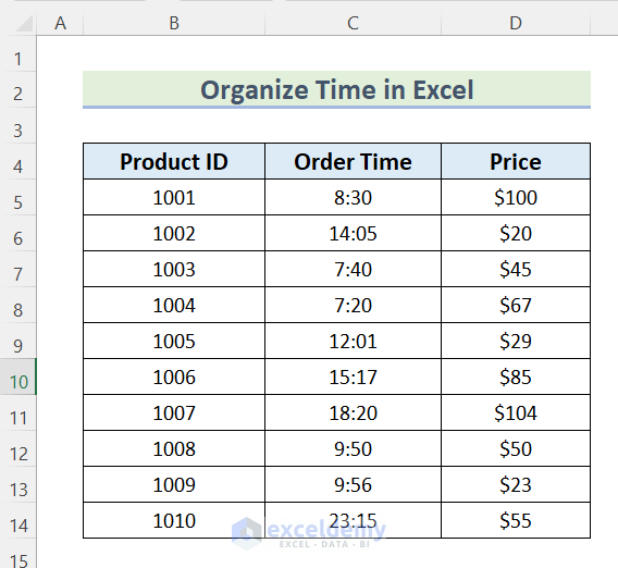
Here, we have a dataset containing the Product ID, Order Time and Price of some products in a factory. We will show you how to organize time in this dataset.

1. Using Direct Drop-Down Option to Organize Time

In the first method, we will use the Direct Drop-Down Option to organize time in the dataset. Follow the steps given below to do it on your own.

Steps:

• First, select Cell range B4:D14.
• Then, go to the Data tab >> click on Sort & Filter >> select Filter.

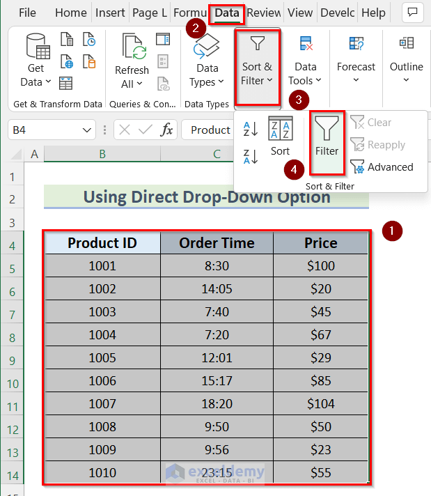
• After that, click on the Drop-Down option that appeared in the Order Time column.
• Then, select Sort Smallest to Largest.

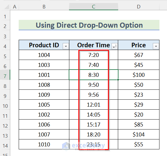
• Now, you can see the organized time in the dataset.

Read More: How to Organize Data for Analysis in Excel (5 Useful Methods)

2. Use of Custom Sort Option to Organize Time in Excel

We can also use the Custom Sort option to sort time in Excel. Go through the following steps to do it on your own dataset.

Steps:

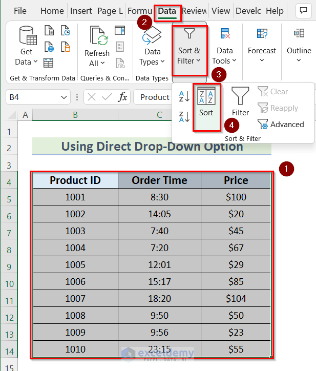
• In the beginning, select Cell range B4:D14.
• Then, go to the Data tab >> click on Sort & Filter >> select Sort.

• Now, the Sort dialog box will open.
• Then, select Order Time in the Sort by box.

• After that, select in the Order box and select Smallest to Largest.
• Then, press OK.

• Finally, you will get the dataset sorted by time.

Read More: How to Organize Raw Data in Excel (6 Easy Methods)

3. Using Pivot Table Feature to Organize Time

Pivot Tables are normally used to summarize the dataset in an understandable way. We can use this feature to organize time in our dataset. Follow the steps given below to use the Pivot Table feature to organize time in your dataset.

Steps:

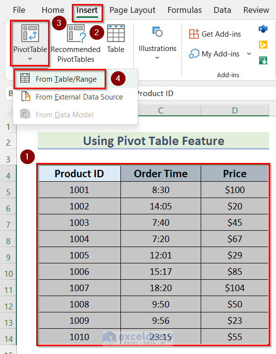
• First, select Cell range B4:D14.
• Then, go to Insert >> click on Pivot Table >> select From Table/Range.

• After that, PivotTable from table or range box will open.
• Here, you can see that the Table/Range is already selected.
• Next, select New Worksheet
• Then, press OK.

• Then, put the Order Time in the Rows area and Product ID in the Values area.

• After that, click on Sum of Product ID.
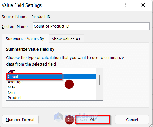
• Then, select Value Field Settings.

• Now the Value Field Settings box will open.
• Here, select Count.
• Then, press OK.

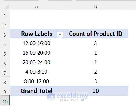
• Now, you will get the Pivot Table organized by time.

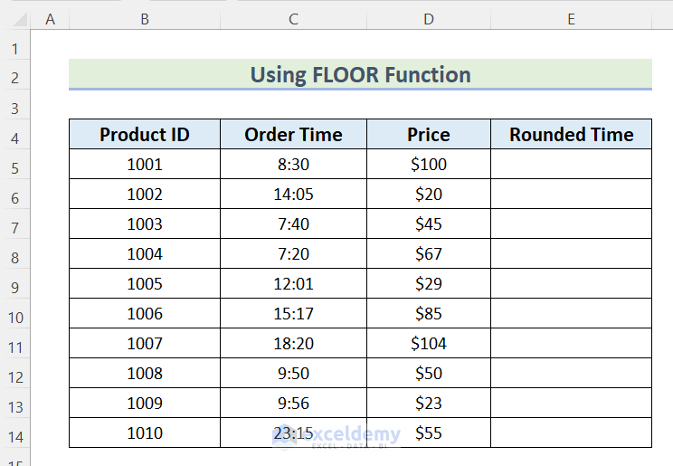
4. Using FLOOR Function to Organize Time in Excel

Here, we will use the FLOOR function to organize time in Excel. The FLOOR function is used to round down a number in the given specified significance.

Follow the steps given below to do it on your own dataset.

Steps:

• First, select the Cell E5.
• Then insert the following formula.

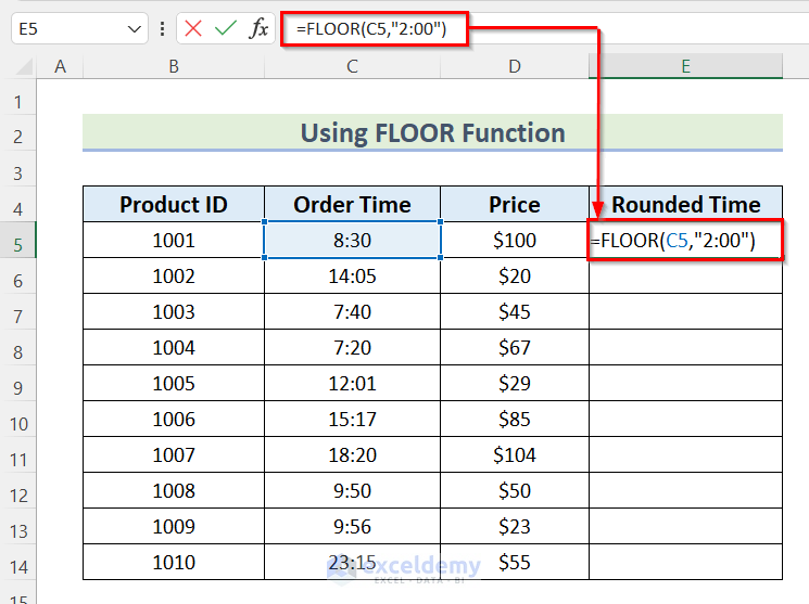
Here, in the FLOOR function, we selected Cell C5 as the number and used the value “2:00” as significance.

• After that, press ENTER to get the value of Rounded Time.
• Then, drag down the Fill Handle tool to AutoFill the formula for the rest of the cells.

• Thus, you will get the Order Time converted into Rounded Time.

• Next, follow the steps of Method_3 to insert the PivotTable.
• Now, we will select the columns in PivotTable Fields.
• Here, put the Rounded Time in the Rows area and Product ID in the Values area.

• After that, click on Sum of Product ID.
• Then, select Value Field Settings.

• Now, the Value Field Settings box will open.
• Then, select Count.
• After that, press OK.

• Finally, you will get the Pivot Table organized by time using the FLOOR function.

5. Applying VLOOKUP Function to Organize Time in Excel

In the final method, we will apply the VLOOKUP function to organize time in Excel. This function is used to look for a value from a given table or range.

Here, we have an additional table containing the Lower Range and Range to group the Order Time.

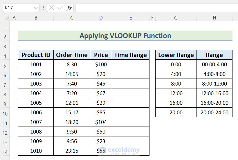
Go through the following steps to do it on your own.

Steps:

• First, select the Cell E5.
• Then, insert the following formula.

Here, in the VLOOKUP function, we selected Cell C5 as lookup_value, selected Cell G5:H10 as table_array, and 2 as column_index_number from where the value of the Time Range will be extracted. Then, TRUE as range_lookup to get the Approximate Match.

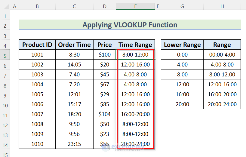
• After that, press ENTER to get the values of the Time Range.

• Next, follow the steps of Method_3 to insert the PivotTable.
• Now, we will select the columns in PivotTable Fields.
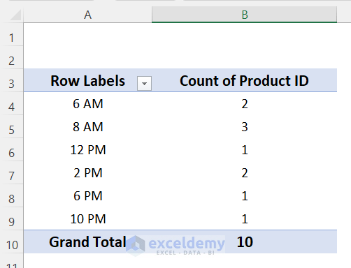
• Here, put the Time Range in the Rows area and Product ID in the Values area.

• After that, click on Sum of Product ID.
• Then, select Value Field Settings.

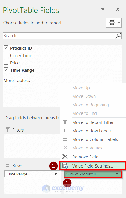
• Now, the Value Field Settings box will open.
• Then, select Count.
• After that, press OK.

• Finally, you will get the Pivot Table organized by time using the VLOOKUP function.

Things to Remember

• In case of using Pivot Table, you can only use up to 500,000 records.
• Again, Pivot Table can add up to 20 Fields as Rows and 20 Fields as Column.
• The FLOOR function returns the #VALUE! Error when the number value is non-numeric.
• The VLOOKUP function returns a #N/A Error when the given formula can’t find what it’s been asked to look for.

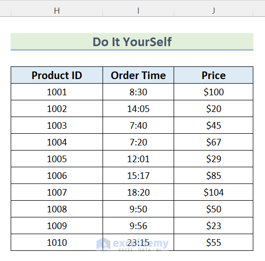
Practice Section

In the article, you will find an Excel workbook like the image given below to practice on your own.

Conclusion

So, in this article, we have shown you how to organize time in Excel. I hope you found this article interesting and helpful. If something seems difficult to understand, please leave a comment. Please let us know if there are any more alternatives that we may have missed. And, visit ExcelDemy for many more articles like this. Thank you!

Related Articles

• How to Organize Expenses in Excel (3 Templates)
• How to Organize Things Alphabetically in Excel (4 Methods)
• Organize Bank Statements in Excel (2 Handy Methods)
• How to Organize Data in Excel from Lowest to Highest (with Quick Steps)
• How to Organize Information in Excel (2 Circumstances)
• How to Organize Sales Leads in Excel (with Quick Steps)