If you are looking for some special tricks to organize sales leads in Excel, you’ve come to the right place. There is one way to organize sales leads in Excel. This article will discuss every step of this method to organize sales leads in Excel. Let’s follow the complete guide to learn all of this.
How to Organize Sales Leads in Excel: Step-by-Step Procedure
In the following section, we will use one effective and tricky method to organize sales leads in Excel. To organize more understandable sales leads, it is necessary to make a basic outline and calculations with formulas and calculate the monthly weighted forecast. This section provides extensive details on this method. You should learn and apply all of these to improve your thinking capability and Excel knowledge. We use the Microsoft Office 365 version here, but you can utilize any other version according to your preference.
Step 1: Create Primary Outline
To organize sales leads in Excel, we have to follow some specified rules. At first, we want to make a dataset. To do this we have to follow the following rules.
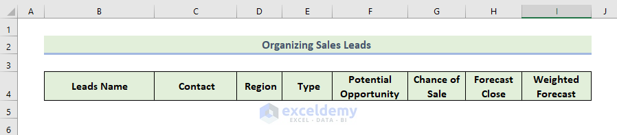
- Firstly, write ‘Organizing Sales Leads’ in some merged cells at a larger font size, That will make the heading more attractive. Then, type your required Headline fields for your data. Click here to see a screenshot that illustrates what the fields look like.
Step 2: Input Data of Sales Leads
Now, after completing the heading part, you have to input the basic information of the sales lead. To do this, you have to follow the following procedures.
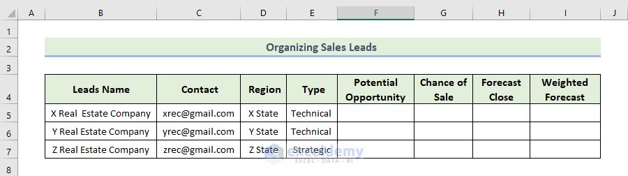
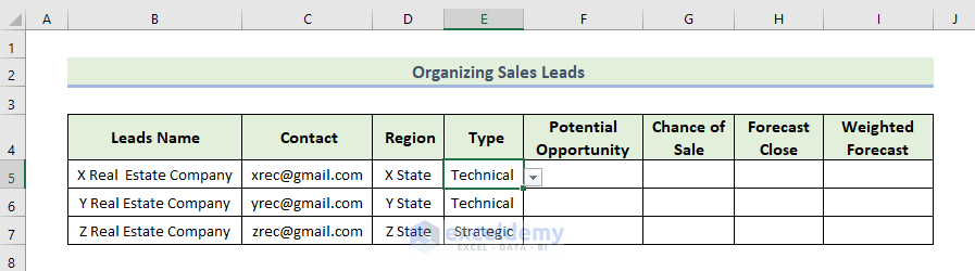
- In the following image, we can see the basic outlines of the sales leads data and its related dataset.
- Here, we have Leads Name, Contact, Region, and Type columns in the following dataset.
- In the Leads Name column, we enter each company name.
- Then, in the Contact column, we type each company’s contact information.
- Next, in the Region column, we enter each company located.
- Then, in the Type column, we type each company’s business type information.
- Next, we want to create a drop-down arrow in the Region. To do this, go to the Data tab, and go to the Data Tools group. Then, select Data Validation.
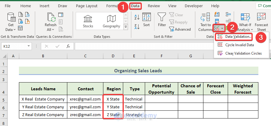
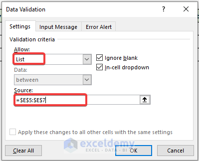
- When the Data Validation dialog box appears, select List in the Allow section and select the Region column’s cells as a range of cells in the Source box. Click on OK.

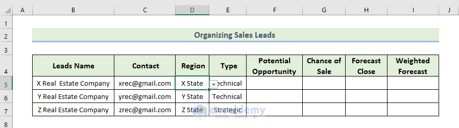
- As a consequence, you will get the following drop-down arrow in Region.
- Next, we want to create a drop-down arrow in the Type. To do this, go to the Data tab. From the Data Tools group, select Data Validation.

- When the Data Validation dialog box appears, select List in the Allow section and select the Type column’s cells as a range of cells in the Source box. Click on OK.
- As a consequence, you will get the following drop-down arrow in Type.
- We will now type in the Potential Opportunity column the value of the sale to the specified company that our product will be able to generate.
- After that, we will type each company’s chances of a sale in the Chance of Sale column.
- Next, in the Forecast Close column, we will type the estimated forecasting time.

Step 3: Calculate Weighted Forecast
Now we are going to calculate the weighted forecast for each company. The weighted forecast allows us to estimate the expected revenue from the sales pipeline. To do this, you have to follow the following process. Here, we will use the SUM function total calculate the total weighted forecast.
- To calculate the weighted forecast, we have to use the following formula in cell I5.
=F5*G5
- Then, press Enter.
- As a result, you will have the weighted forecast for the first company in the dataset.

- Next, drag the Fill Handle icon to fill out the rest of the cells in the column with the formula.
- As a consequence, you will get the weighted forecast for all the entries of the dataset.

- Next, you have to add a new row to calculate the total values of the Potential Opportunity and Weighted Forecast columns.
- To calculate the total potential opportunity, we have to use the following formula in cell F8.
=SUM(F5:F7)
- Then, press Enter.
- As a consequence, you will get the total value as shown below.

- To calculate the total weighted forecast, we have to use the following formula in cell I8.
=SUM(I5:I7)
- Then, press Enter.
- As a consequence, you will get the total value as shown below.

Step 4: Calculate Monthly Weighted Forecast to Organize Sales Leads
Now, we are going to calculate the monthly weighted forecast to organize sales leads in Excel. To do this you have to follow the following process. Here, we will use the SUM function total calculate the total weighted forecast.
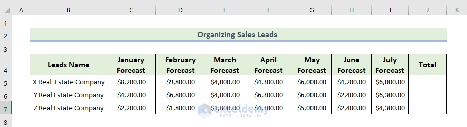
- First of all, you have to enter the first six months’ forecast value for each company as shown below.
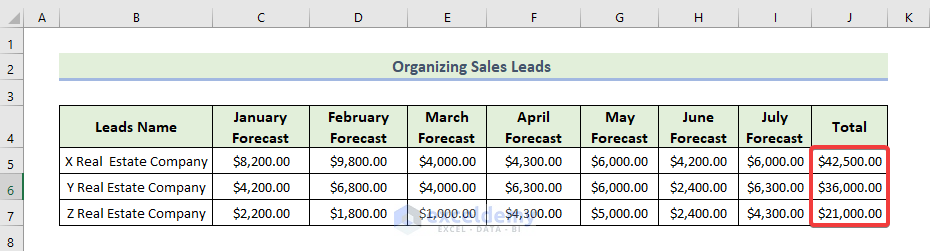
- To calculate the total weighted forecast for X Real Estate Company, we have to use the following formula in cell J5.
=SUM(C5:I5)
- Then, press Enter.
- As a consequence, you will get the total weighted forecast for X Real Estate Company, as shown below.

- Next, drag the Fill Handle icon to fill out the rest of the cells in the column with the formula.
- Therefore, you will get the total weighted forecast for each company, as shown below.
- Now, we are going to create a 3-D Pie chart for presenting sales leads.
- To create a Pie chart, select the range of data and go to the Insert tab. Next, select the 3-D Pie chart.

- As a consequence, you will get the following chart.

- To modify the chart style, select Chart Design and then, select your desired Style7 option from the Chart Styles group.
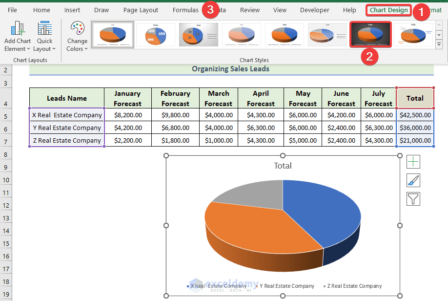
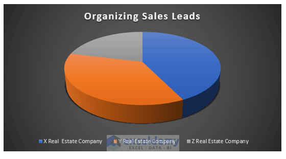
- Therefore, you will get the following 3-D Pie chart.
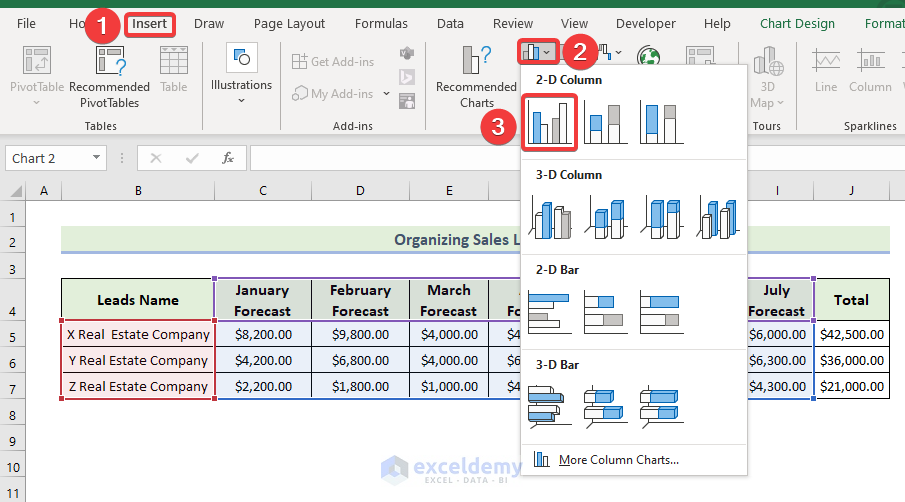
- Now, we are going to create a Clustered Column chart for presenting monthly weighted forecasts.
- To create a chart, select the range of data and go to the Insert tab. Next, select the Clustered Column chart.
- As a consequence, you will get the following chart.

- To modify the chart style, select Chart Design and then, select your desired Style8 option from the Chart Styles group.
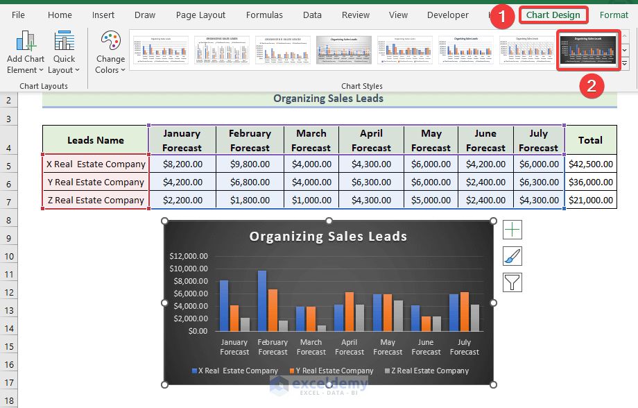
- Therefore, you will get the following Clustered Column chart.

- As a consequence, you will get the final output like the following.

Read More: How to Organize Expenses in Excel
Download Practice Workbook
Download this practice workbook to exercise while you are reading this article. It contains all the datasets in different spreadsheets for a clear understanding. Try yourself while you go through the step-by-step process.
Conclusion
That’s the end of today’s session. I strongly believe that from now you may be able to organize sales leads in Excel. If you have any queries or recommendations, please share them in the comments section below.
Related Articles
- How to Organize Raw Data in Excel
- How to Organize Data for Analysis in Excel
- How to Organize Data in Excel from Lowest to Highest
- How to Organize Information in Excel
- How to Organize Time in Excel
- How to Organize Things Alphabetically in Excel
<< Go Back to Organize Data in Excel | Data Analysis with Excel | Learn Excel
Get FREE Advanced Excel Exercises with Solutions!
