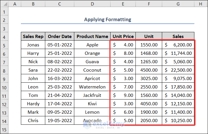
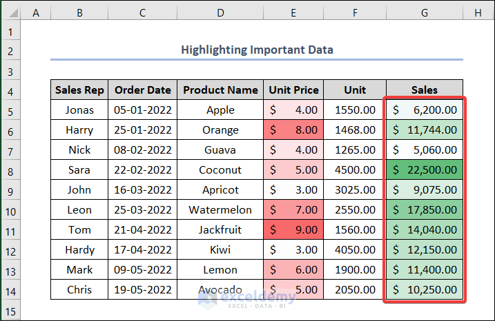
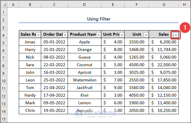
The dataset showcases a Sales Report of Sales reps containing Product Name, Unit Price, Units sold, and Sales amount.
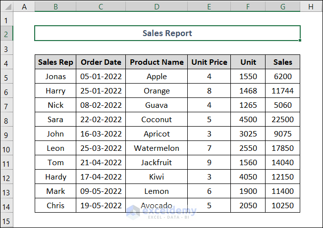
Example 1 – Applying Formatting
Steps:
- Select columns E and G.
- Go to the Home tab and select the $ sign Number.
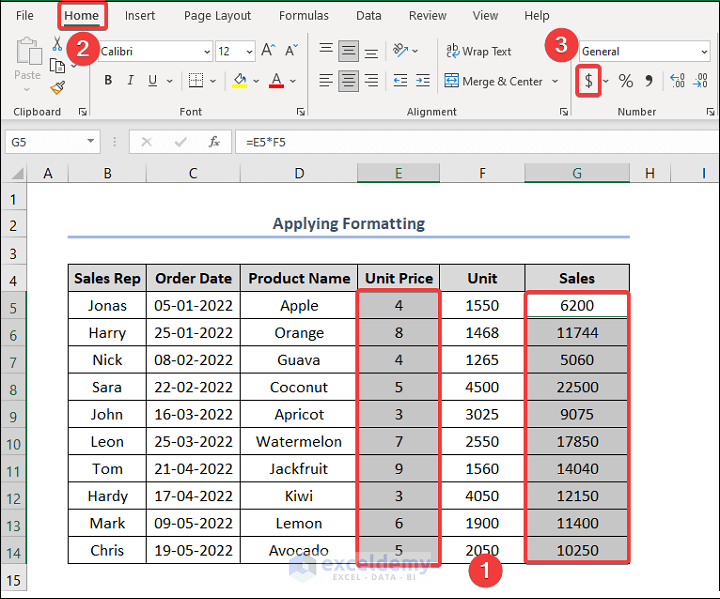
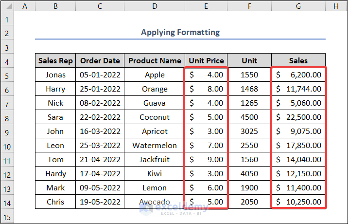
Unit Price and Sales are in Accounting format.
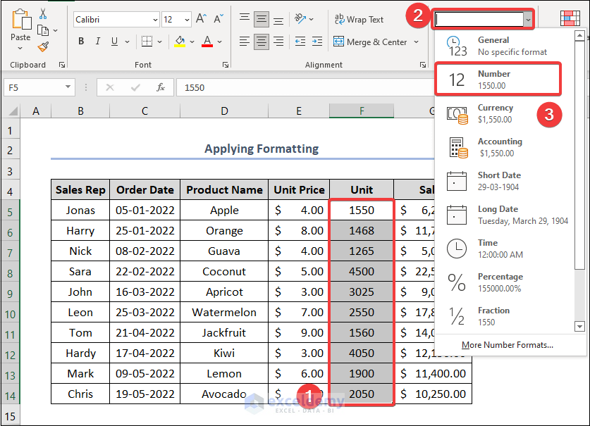
Column F contains Units sold by respective Sales Reps. Format the data as Number:
- Select F5:F14.
- In Number, choose Number format.
This is the output.
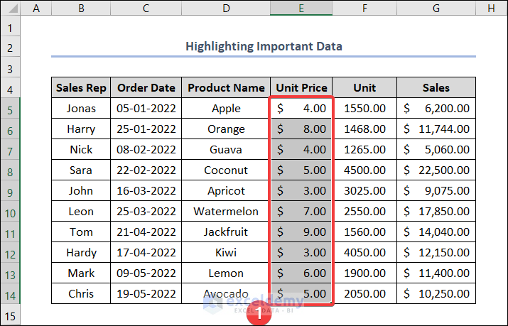
Example 2 – Highlighting Cells
Steps:
- Select E5:E14.
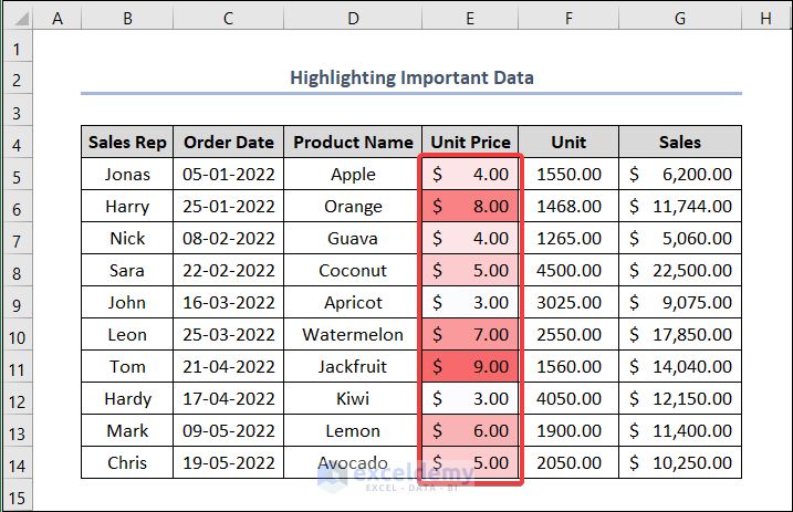
- Go to the Home tab and select Conditional Formatting > Colour Scales > Red – White Color Scale.
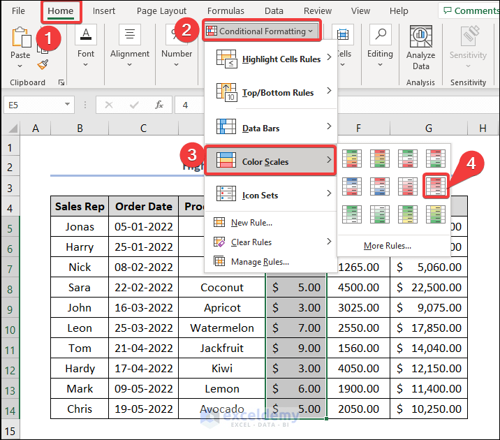
- In Red – White Color Scale, the cell with the maximum value gets a dark red color, and the color fades with decreasing values.
- Apply the same method to column G with the Green – White Color Scale.
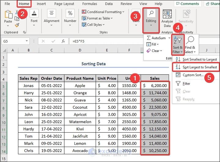
Example 3 – Sorting Raw Data
Steps:
- Select G5:G14.
- Go to the Home tab and select Editing > Sort & Filter > Sort Largest to Smallest.
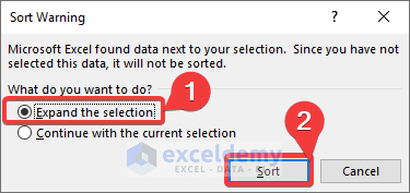
- In the Sort Warning dialog box, Expand the selection is selected automatically.
- Click Sort.
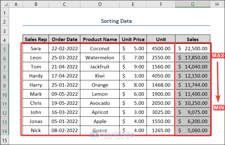
Data is sorted in descending order.
Read More: How to Organize Data in Excel from Lowest to Highest
Example 4 – Using the Filter Option to Organize Raw Data
Steps:
- Use the drop-down arrow beside the Sales header to Filter data.
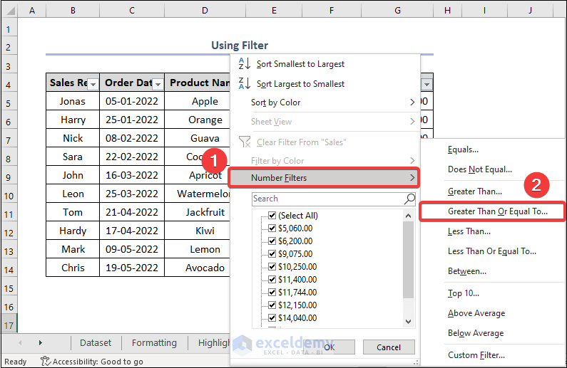
To show the rows with a Sales amount of $10,000 or greater only:
- Select Number Filters > Greater Than or Equal To.
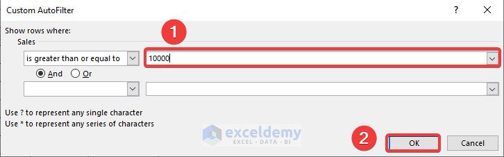
- In the Custom AutoFilter dialog box, enter 10000 and click OK.
- The Sales amounts displayed are greater than $10,000.
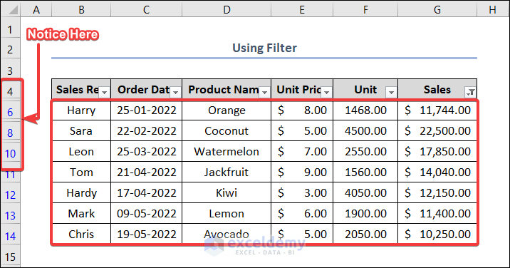
Note: Between rows 4 and 10, there are hidden rows: the Sales amounts are less than $10,000.
Example 5 – Hiding Unimportant Data
Steps:
- Select rows 8 and 13 by clicking the row number.
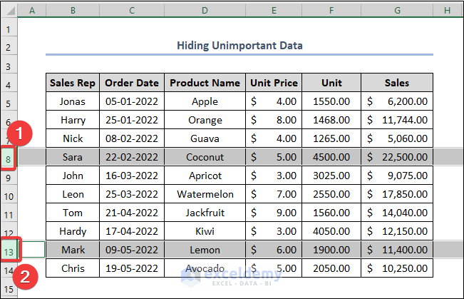
- Go to the Home tab.
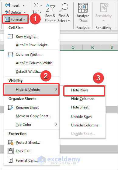
- In Cells, select Format > Hide & Unhide > Hide Rows.
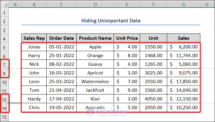
The selected rows are hidden.
Read More: How to Organize Data for Analysis in Excel
Example 6 – Using the FILTER Function to Organize Raw Data in Excel
Create a table with the same headers. To see the details of Apple only:
Steps:
- Select B17. Enter the formula below and press ENTER.
=FILTER(B5:G14,D5:D14=D5,"")
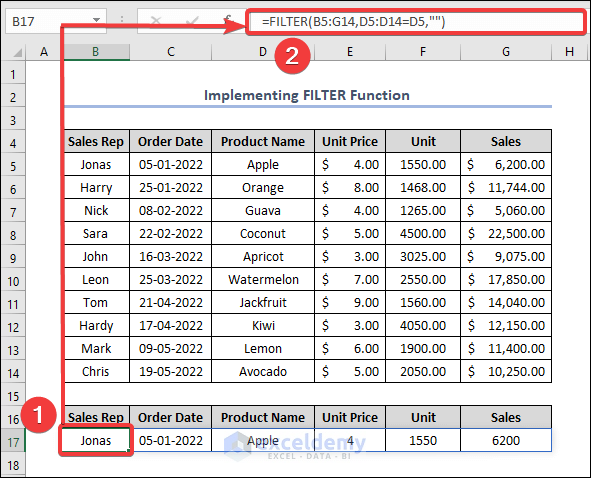
Only the values related to Apple are displayed.
Download Practice Workbook
Download the following Excel workbook.
Related Articles
- How to Organize Information in Excel
- How to Organize Things Alphabetically in Excel
- How to Organize Time in Excel
- How to Organize Expenses in Excel
<< Go Back to Organize Data in Excel | Data Analysis with Excel | Learn Excel
Get FREE Advanced Excel Exercises with Solutions!

I read your entire article. I liked it very much. I have a question, but not related to this topic.
In my business, i’ve 5 sales person working for me in 3 different areas. Now, i wantto know the number of sales p with sales amount less than 350/week.
Help me on this..
Hello DEANNA,
First of all, many many thanks for your appreciation. At the end of the day, these kinds of words motivate us a lot. Now, get back to your query.
For your convenience, download this practice workbook.
Firstly, we’ve created a dataset as per your description. We’ve constructed an imaginary Weekly Sales Report of your company. Let’s see the following picture.
Now, we’ll find out how many sales reps cannot cross the Sales Amount of $350 in a week.
At first, go to cell D11 and enter the following formula into the cell.
=COUNTIF(D5:D9,"<350")Secondly, press the ENTER key.
Here, we can see that Excel returns 2 as result. Because two employees made sales amount below $350 which are Person 2 and Person 5. We think you wanted to know about this part.
As a bonus, we’ll teach you one more trick. You can get a more specific answer with this. Guess, if you wanted to know how many sales reps made sales amount below $350 in a specific zone. Let’s say, in the West zone. Obviously, you can crack this too.
Firstly, select cell D11 and write down the formula below.
=COUNTIFS(D5:D9,"<350",C5:C9,"West")As usual, tap ENTER.
The result is 1 because there is only one Sales Rep in the West zone with a Sales Amount less than $350 who is Person 2.
To explore more about Excel, please visit our website Exceldemy: One-stop Excel solution provider…