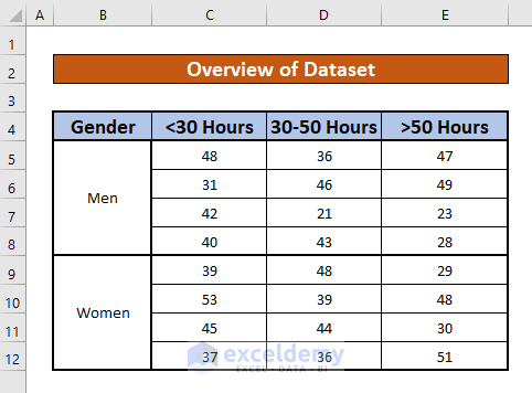
We have a dataset that contains information about several working time of some men and women. We will analyze the quantitative data using the T-Test, F-Test, ANOVA, and a Histogram.
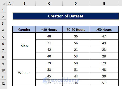
Step 1 – Create a Dataset with Proper Parameters
- We will make a dataset that contains information about working hours of some men and women.
- The column headers separate the groups by the conditions.
- Insert the values manually.
- Note that the Gender cells only have values in B5 and B9 and represent merged cells.
Read More: How to Analyze Qualitative Data in Excel
Step 2 – Enable the Analysis ToolPak Add-in
- Press the File ribbon.
- Select Options (you may need to use the More menu).
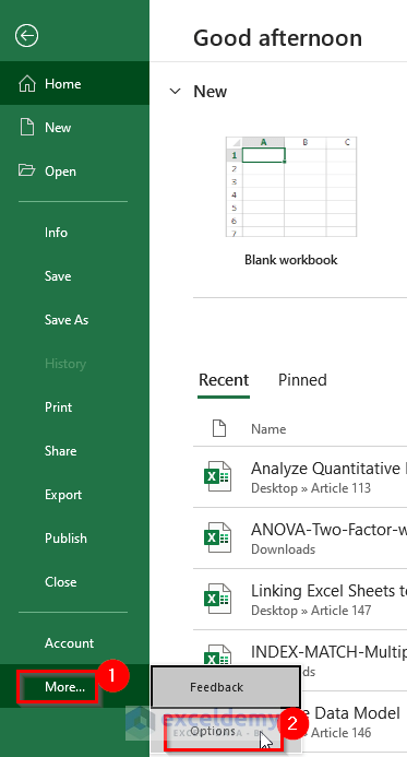
- An Excel Options dialog box will appear.
- Select Add-ins.
- Select Excel Add-ins from the Manage drop-down list.
- Select the GO option.
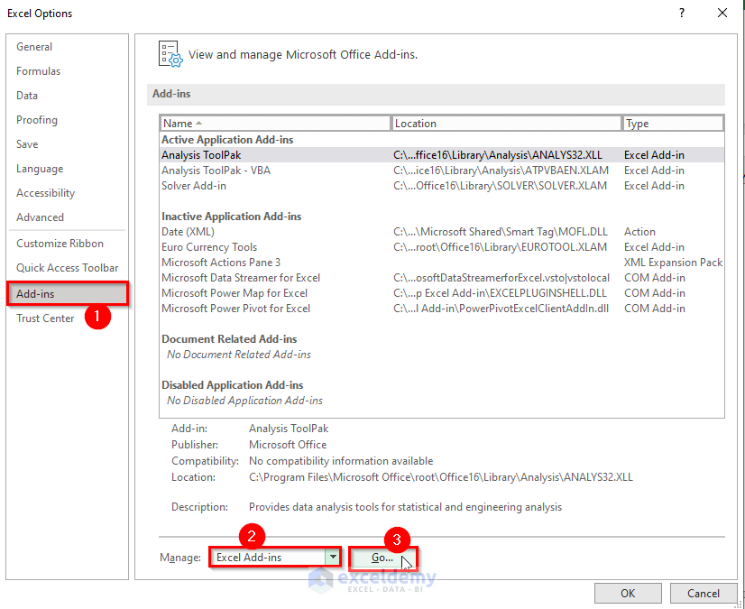
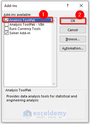
- The Add-ins dialog box will pop up.
- Select Analysis ToolPak and press OK.
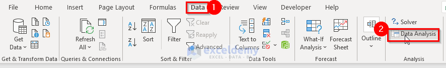
- You will get the Data Analysis command inside the Data ribbon.
Read More: How to Analyse Qualitative Data from a Questionnaire in Excel
Step 3 – Perform a T-Test to Compare Means with Quantitative Data
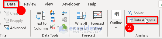
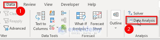
- From your Data tab, go to Analysis and select Data Analysis.
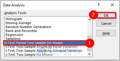
- A Data Analysis dialog box will appear.
- Select t-Test Paired two Sample for Means under the Analysis Tools drop-down list.
- Press OK.
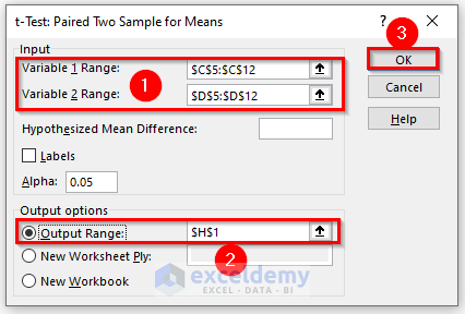
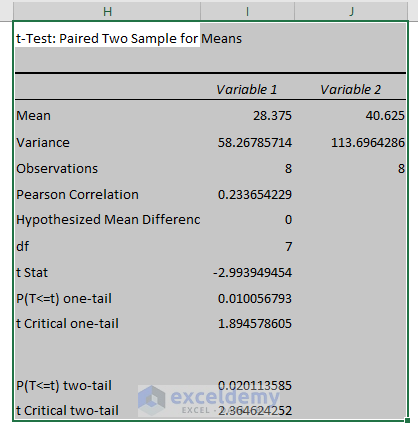
- A t-Test Paired two Sample for Means dialog box pops up.
- Put $C$5:$C$12 in the Variable 1 Range box.
- Put $D$5:$D$12 in the Variable 2 Range box.
- Put $H$1 in the Output Range box and check it.
- Press OK.
- You will get a quantitative data analysis result using a T-Test analysis.
Read More: How to Convert Qualitative Data to Quantitative Data in Excel
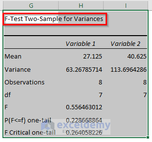
Step 4 – Apply an F-Test Two-Sample for Variances with Quantitative Data
- From your Data tab, go to Analysis and select Data Analysis.
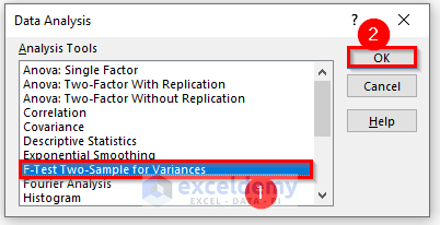
- A Data Analysis dialog box will appear.
- Select F-Test Two-Sample for Variances under the Analysis Tools drop-down list.
- Press OK.
- The F-Test Two-Sample for Variances dialog box pops up.
- Put $C$5:$C$12 in the Variable 1 Range box.
- Put $D$5:$D$12 in the Variable 2 Range box.
- Put $G$1 in the Output Range box and press OK.
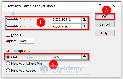
- Here’s the result.
Step 5 – Perform an ANOVA Two-Factor with Replication Analysis
- From your Data tab, go to Analysis and select Data Analysis.
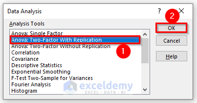
- Select Anova: Two-Factor With Replication under the Analysis Tools drop-down list.
- Press OK.
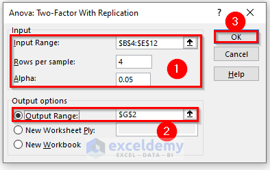
- A dialog box pops up.
- Put $B$4:$E$12 in the Input Range typing box.
- Type 4 in the Rows per sample box.
- Use 0.05 in the Alpha box.
- Put $G$2 in the Output Range box and press OK.
- Here’s the result.
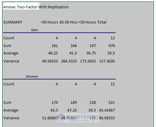
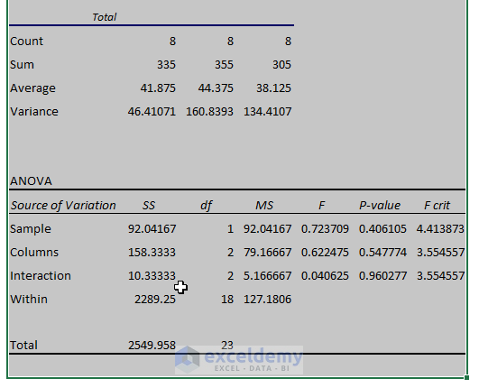
- The rest of the AVONA analysis is like below:
Read More: How to Analyze Raw Data in Excel
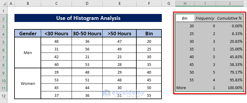
Step 6 – Use a Histogram to Analyze Quantitative Data
- From your Data tab, go to Analysis and select Data Analysis.
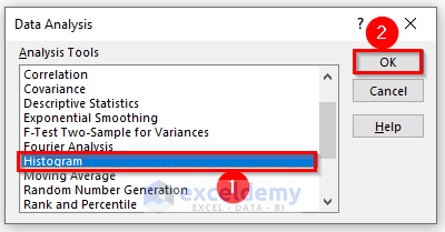
- Select Histogram under the Analysis Tools drop-down list.
- Press OK.
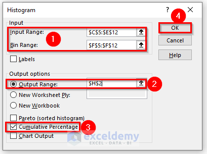
- A Histogram dialog box pops up.
- Put $C$5:$E$12 in the Input Range box.
- Put $F$5:$F$12 in the Bin Range box.
- Put $H$2 in the Output Range box.
- Check the Cumulative Percentage option.
- Press OK.
- You’ll get a chart-like histogram.
Read More: How to Analyze Time Series Data in Excel
Things to Remember
- Press ALT, F, then T to bring up the Excel Options dialog box.
- If a value can’t be found in the referenced cell, the #N/A! error happens in Excel.
- The #DIV/0! error happens when a value is divided by zero(0) or the cell reference is blank.
Download the Practice Workbook
Related Articles
- How to Analyze Large Data Sets in Excel
- How to Analyze Text Data in Excel
- How to Analyze Sales Data in Excel
- How to Analyze Likert Scale Data in Excel
- How to Analyze qPCR Data in Excel
<< Go Back to Data Analysis with Excel | Learn Excel
Get FREE Advanced Excel Exercises with Solutions!
